Download as PPSX, PPTX

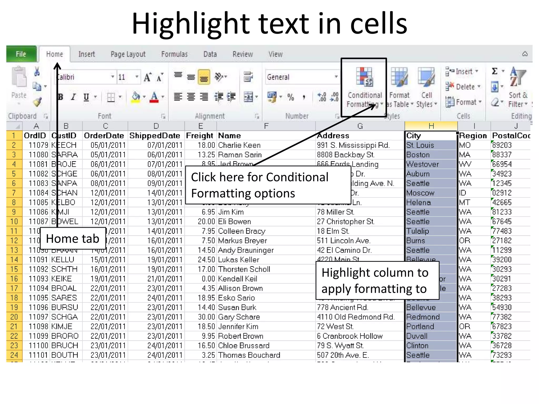

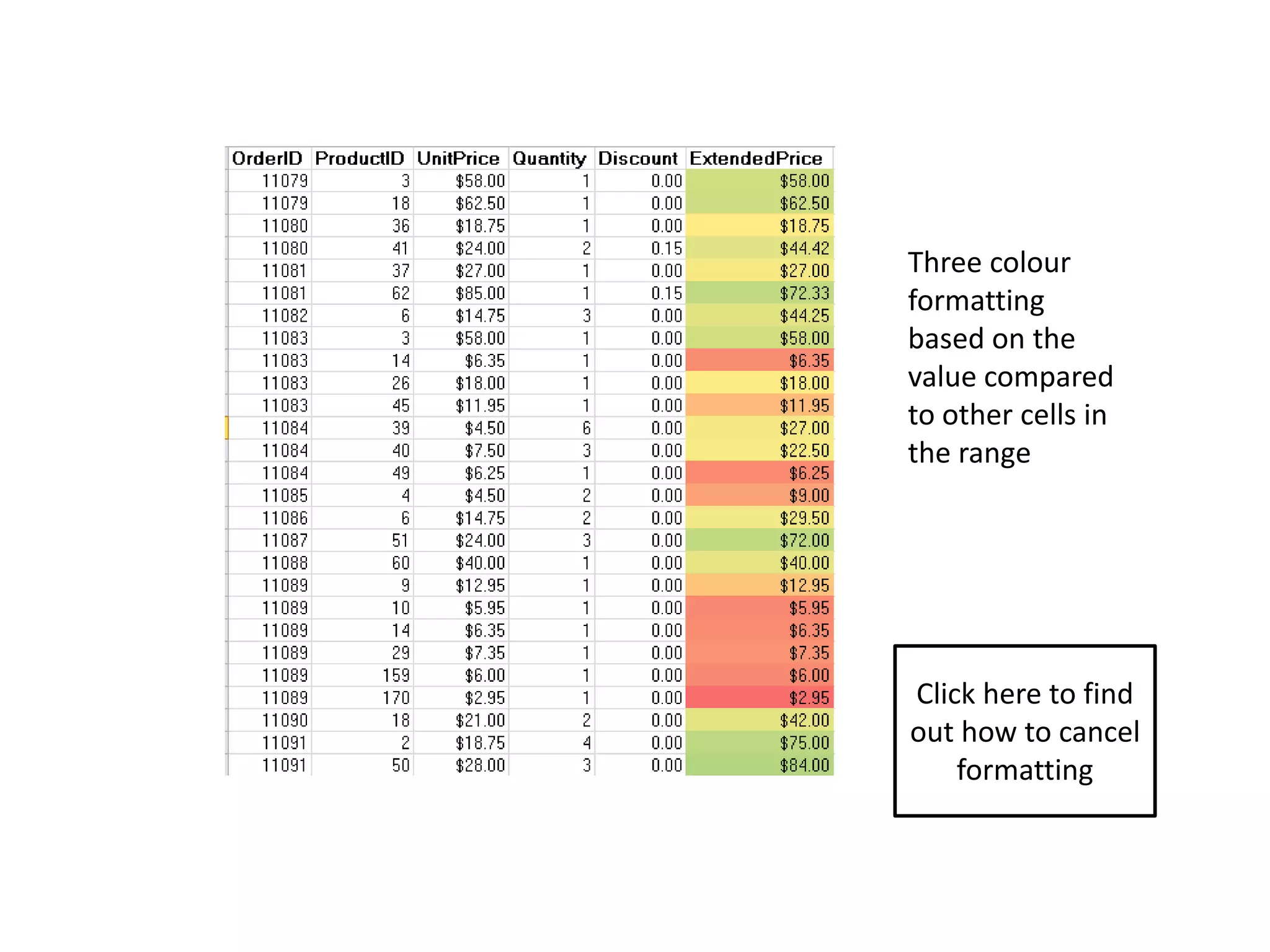

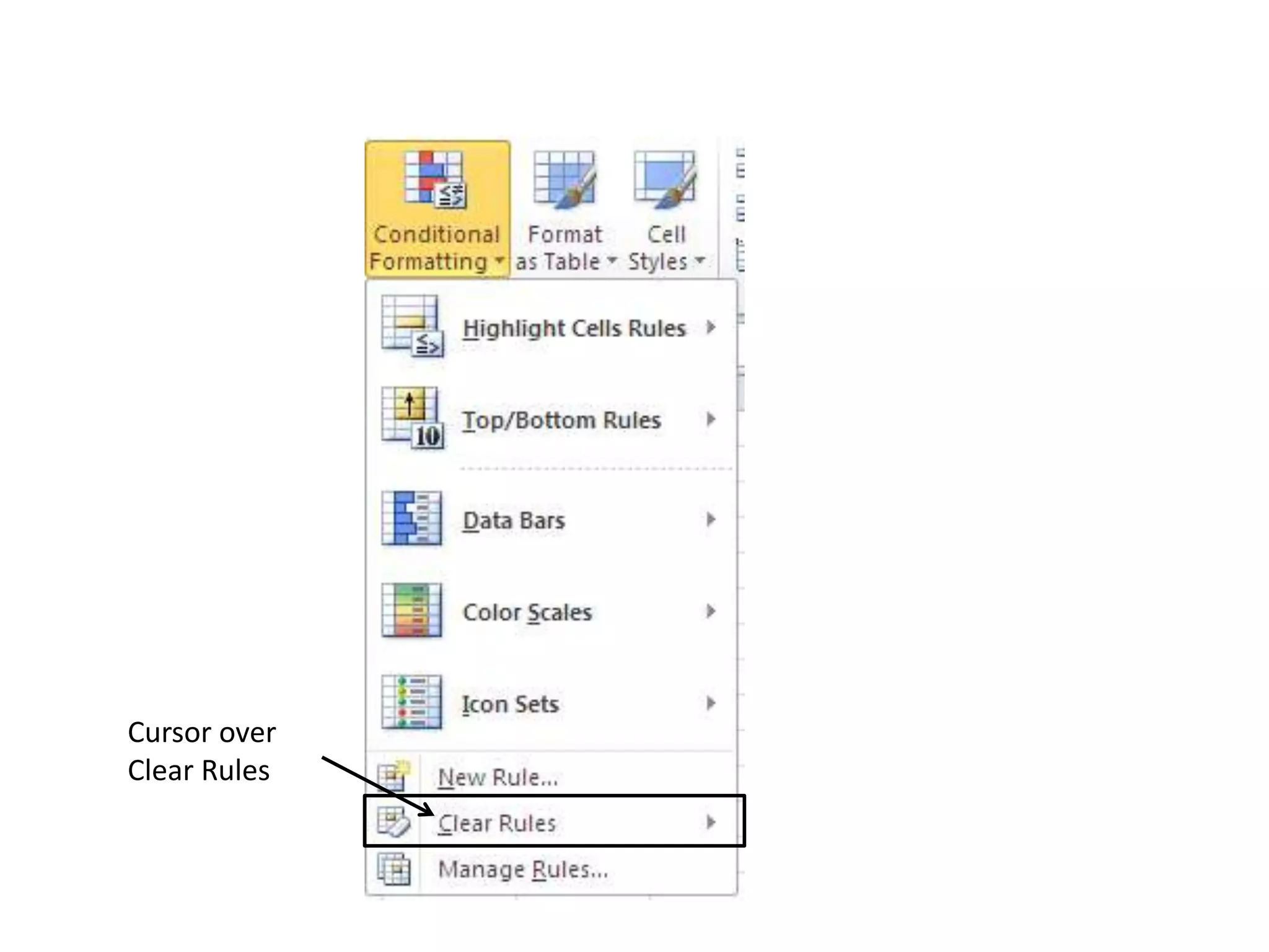
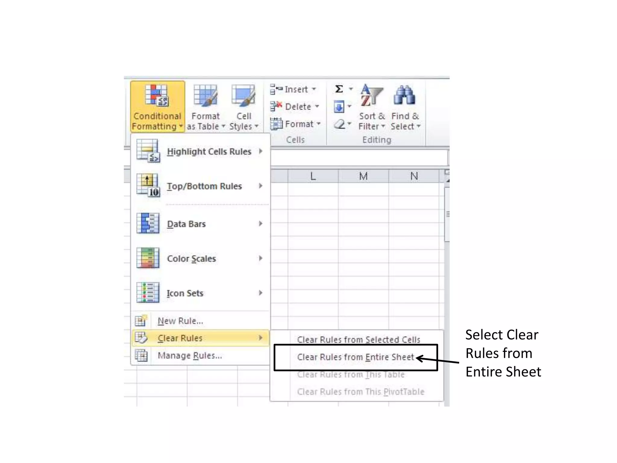
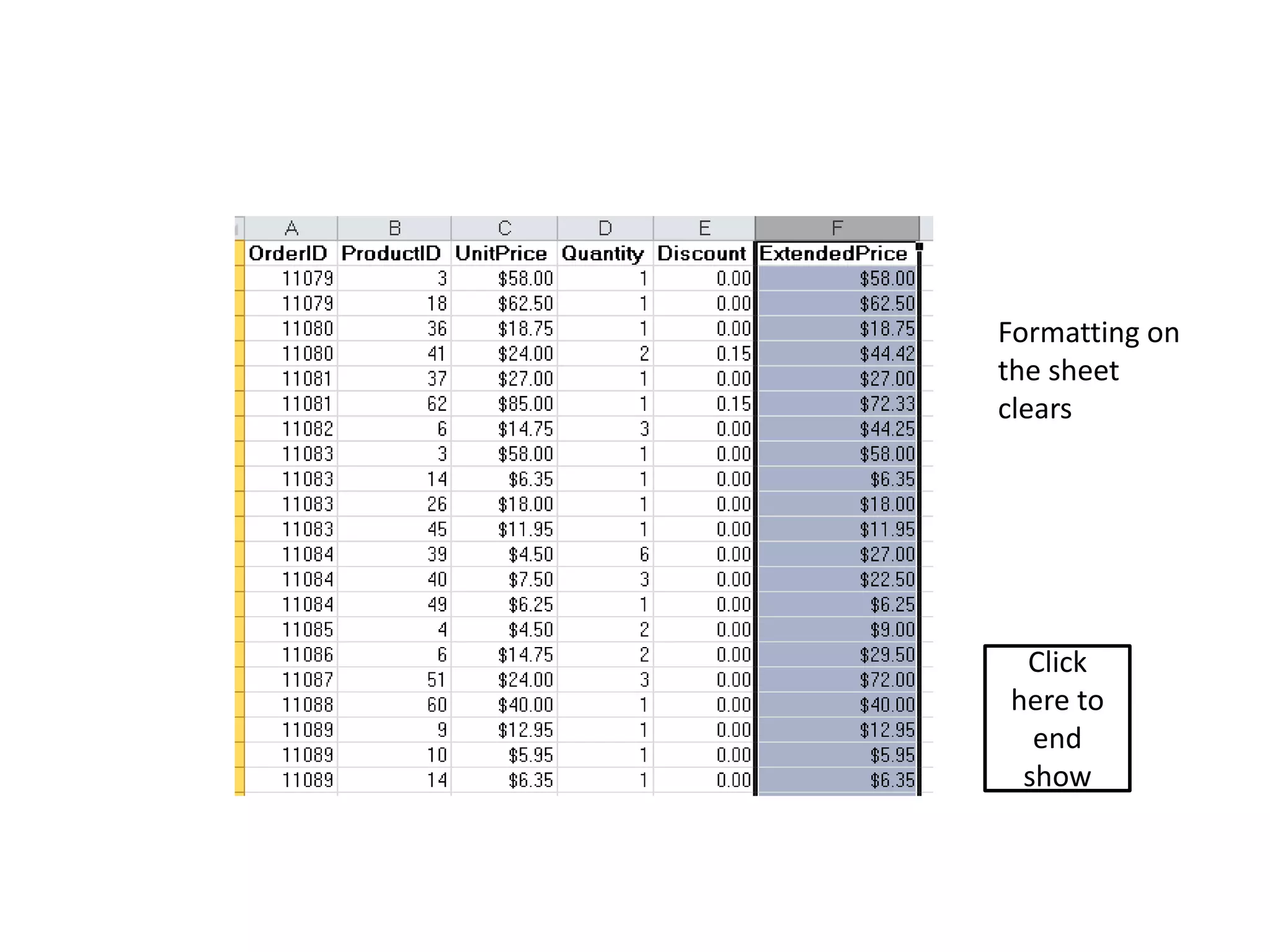
Conditional formatting in Excel allows cells to be formatted based on their data values. This makes spreadsheets easier to read. Formatting options include highlighting text that contains specific words, using color scales to shade cells differently based on values, and more granular controls over formatting styles and values. Conditional formatting rules can be cleared from a sheet by selecting "Clear Rules" under the Conditional Formatting menu.
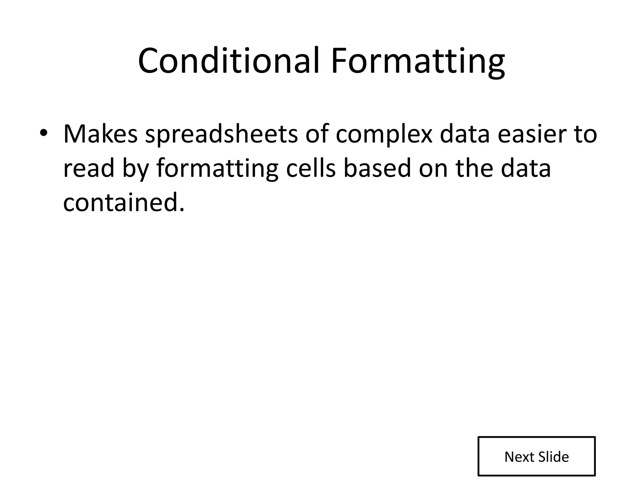
Overview of Conditional Formatting in Excel, making complex data easier to read through specific cell formatting.
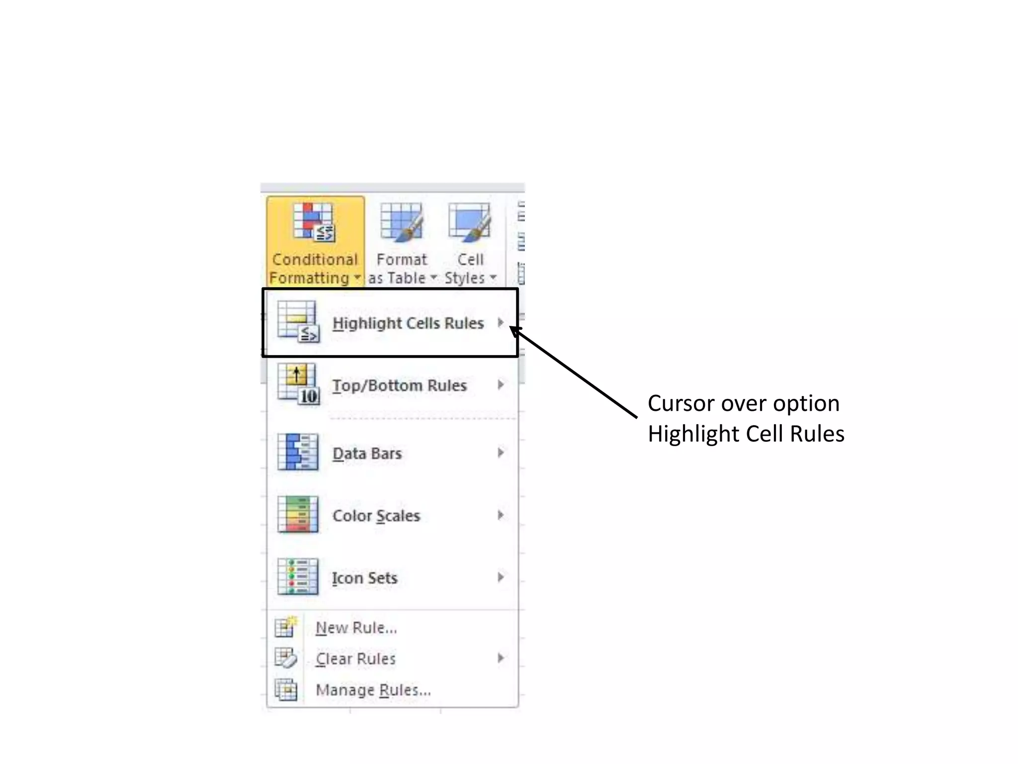
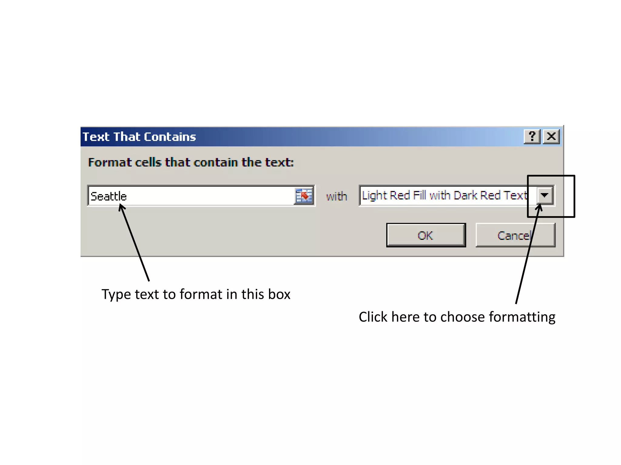
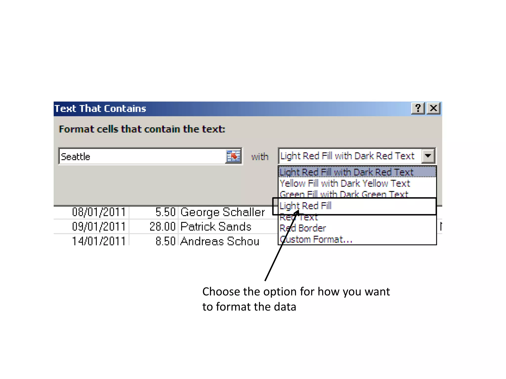
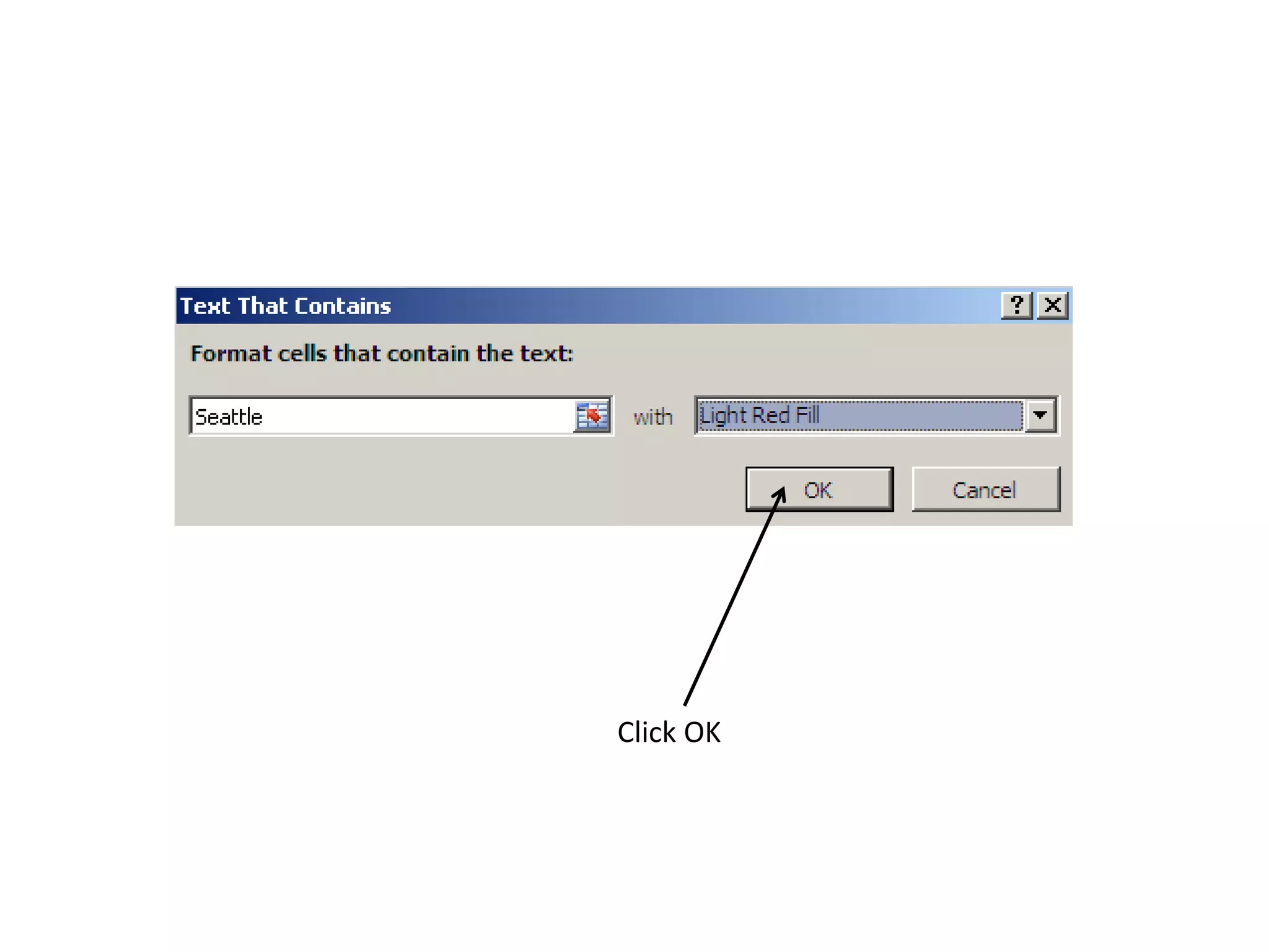
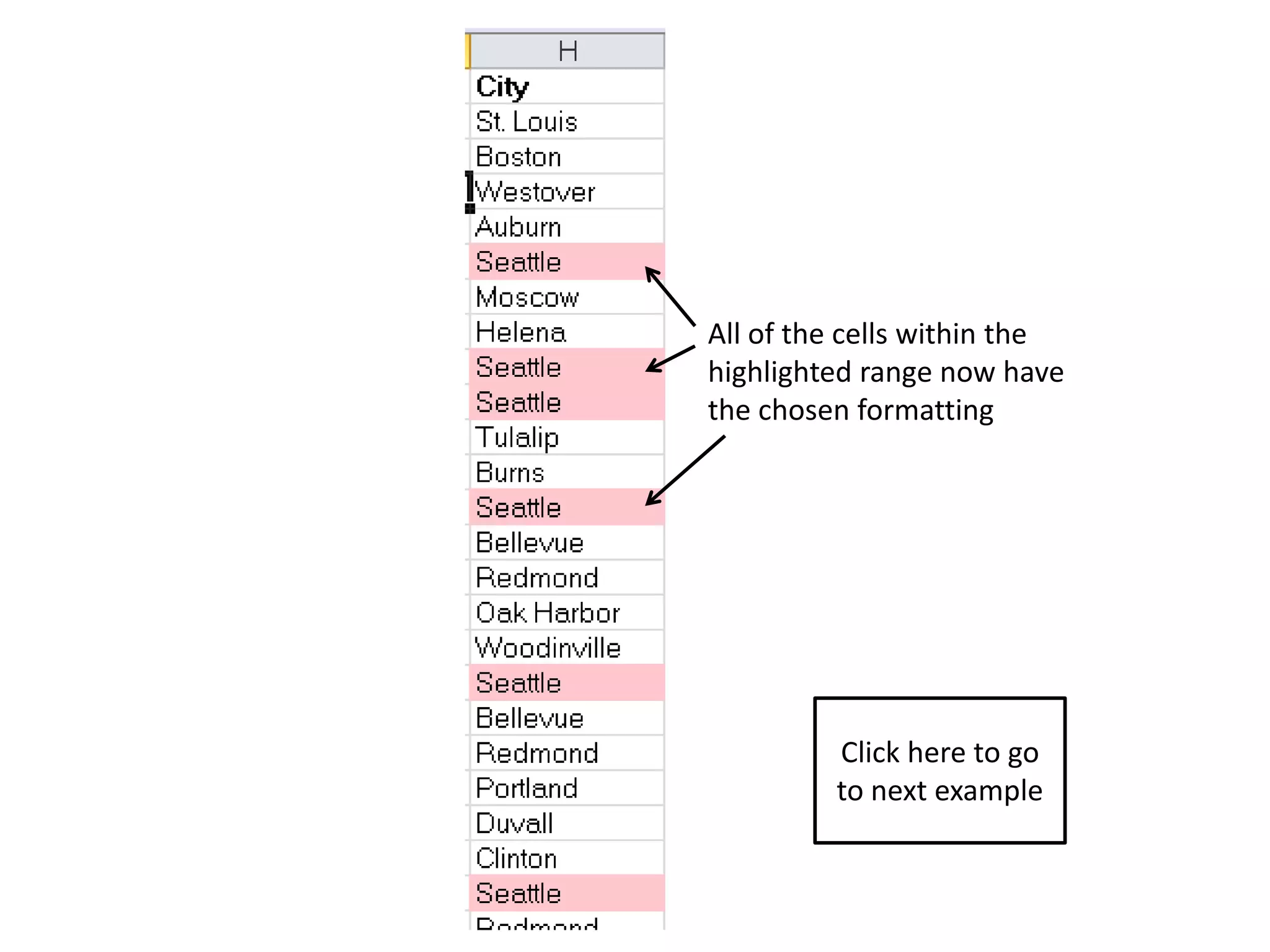
Steps for highlighting text in cells using Conditional Formatting, including how to select text rules and apply chosen formatting.
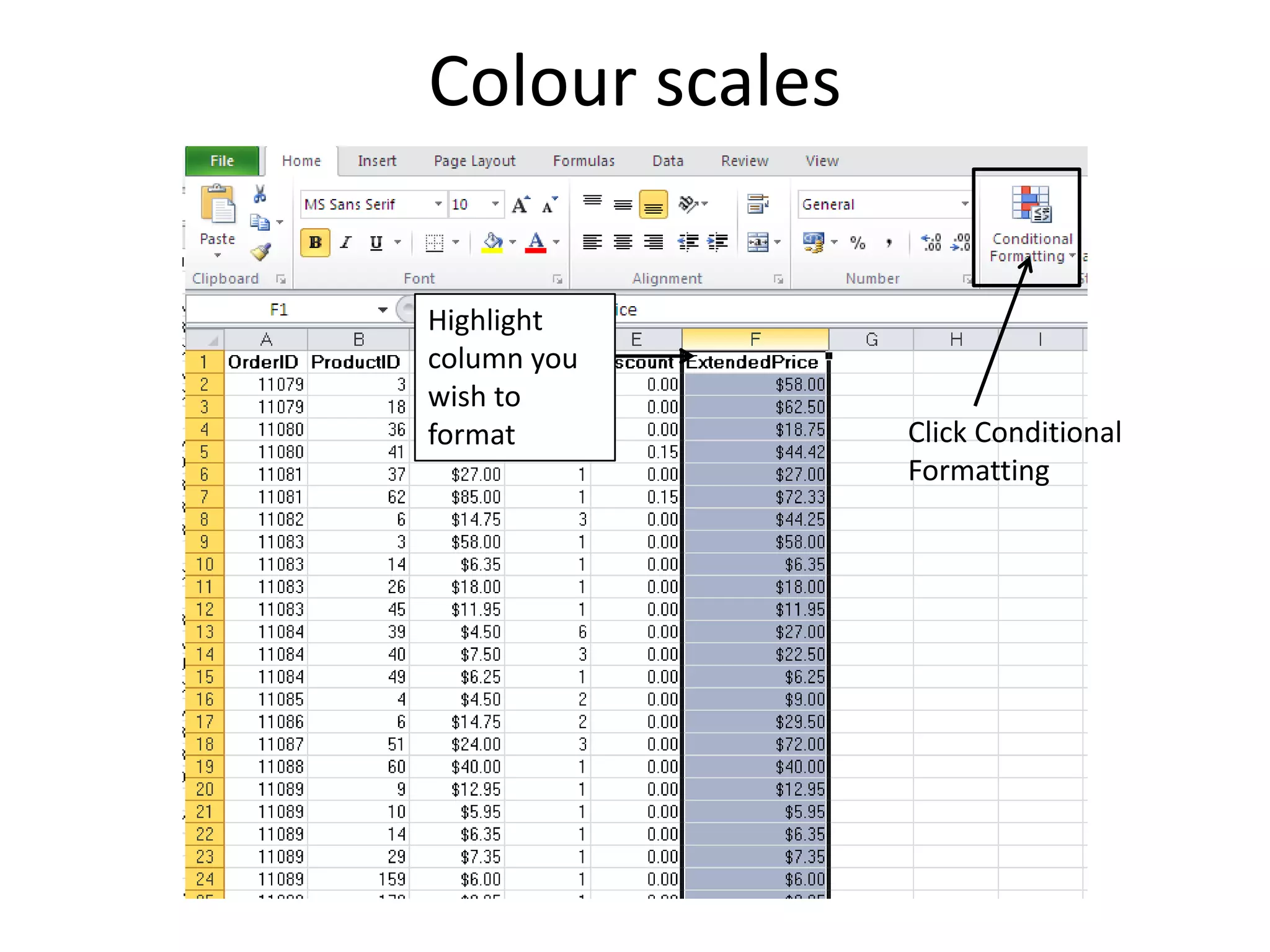
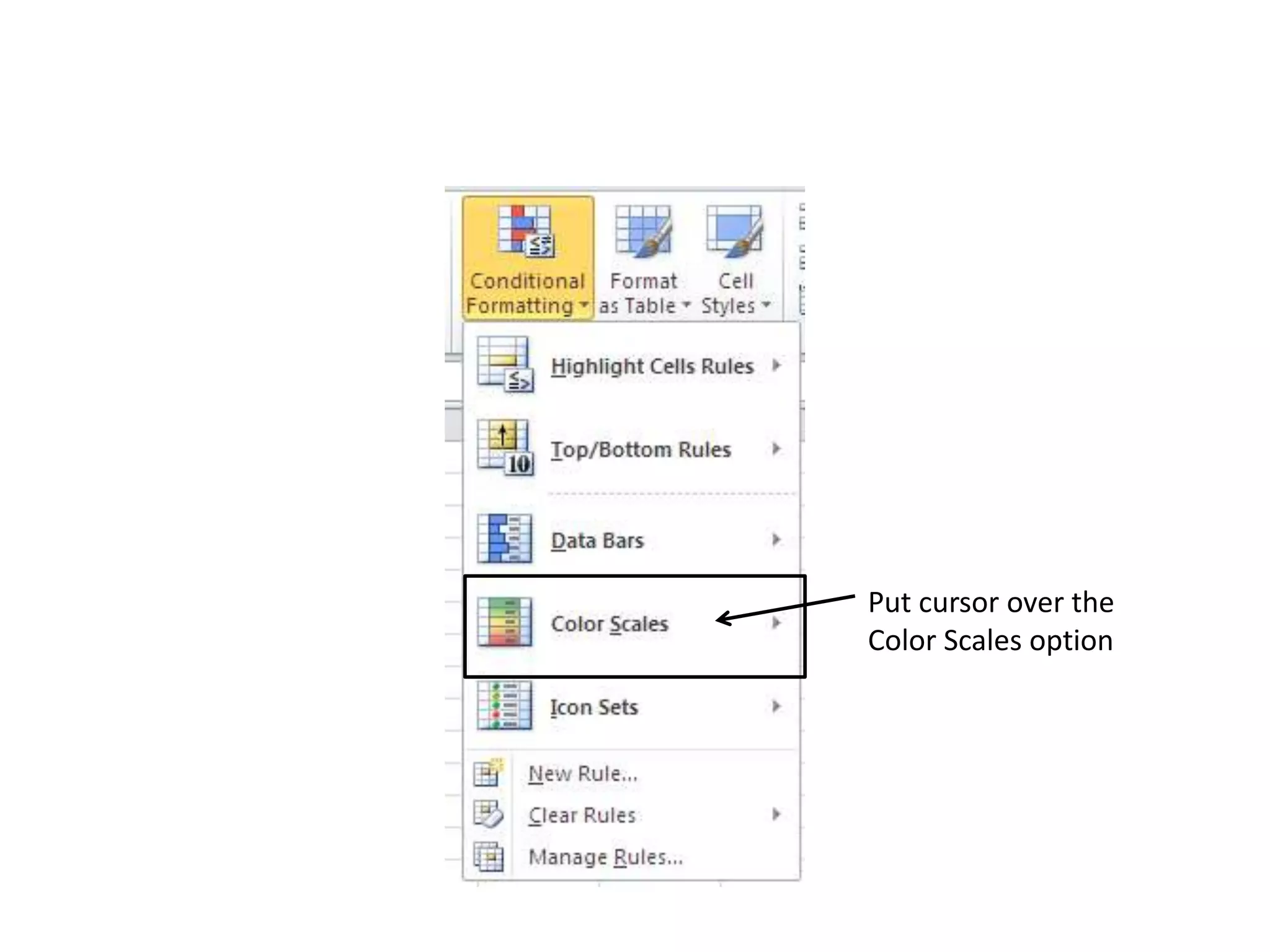
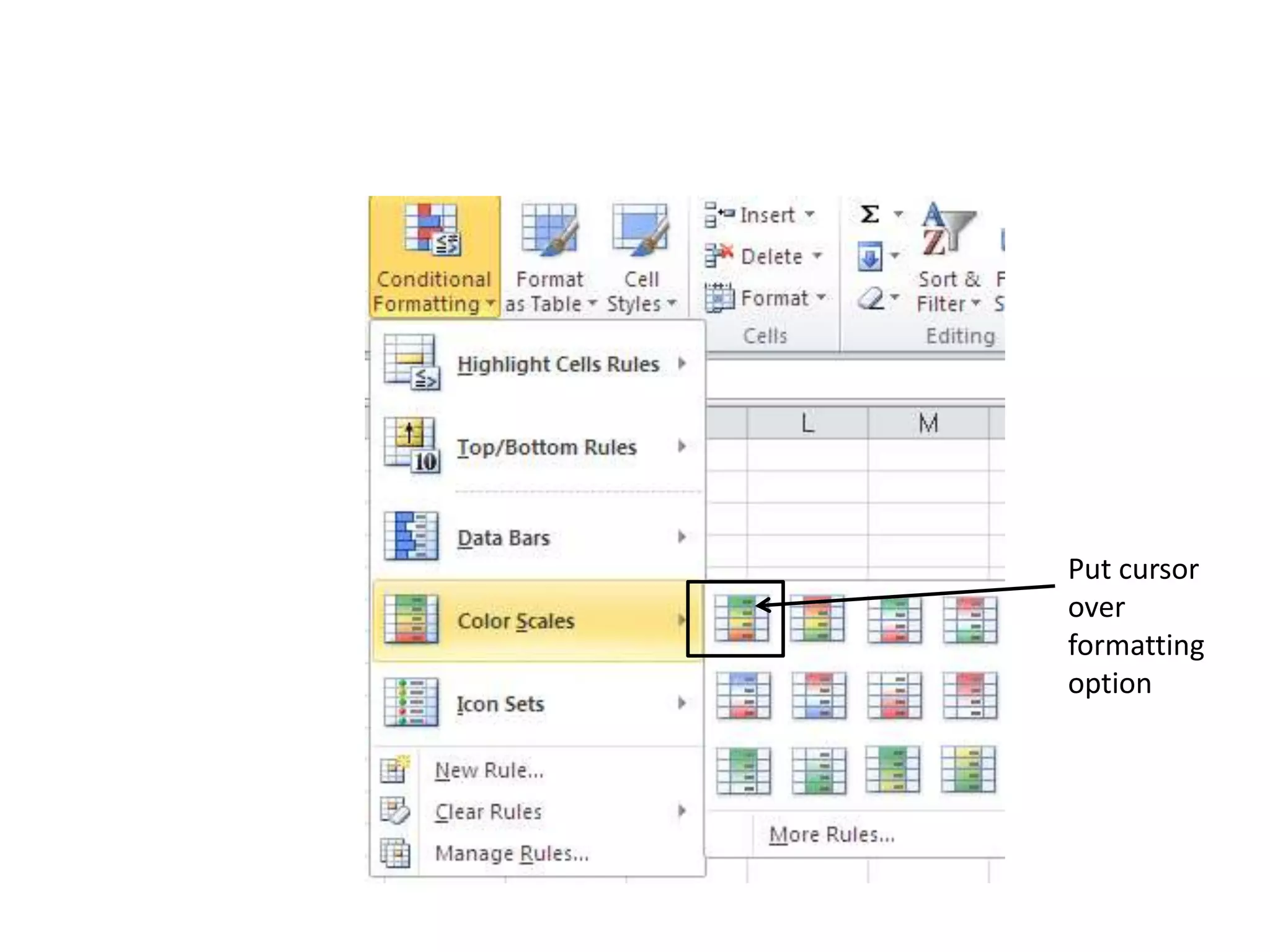
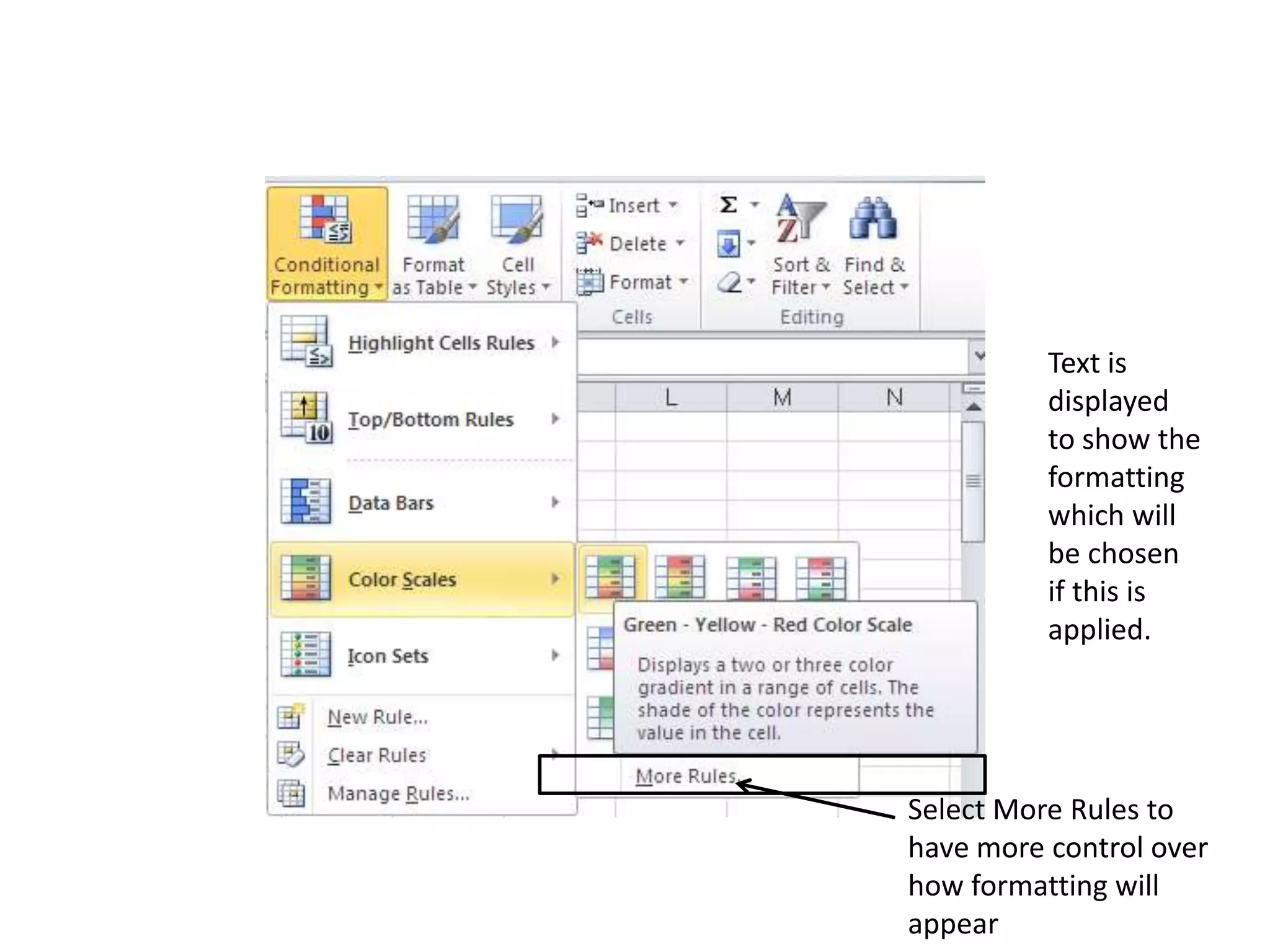
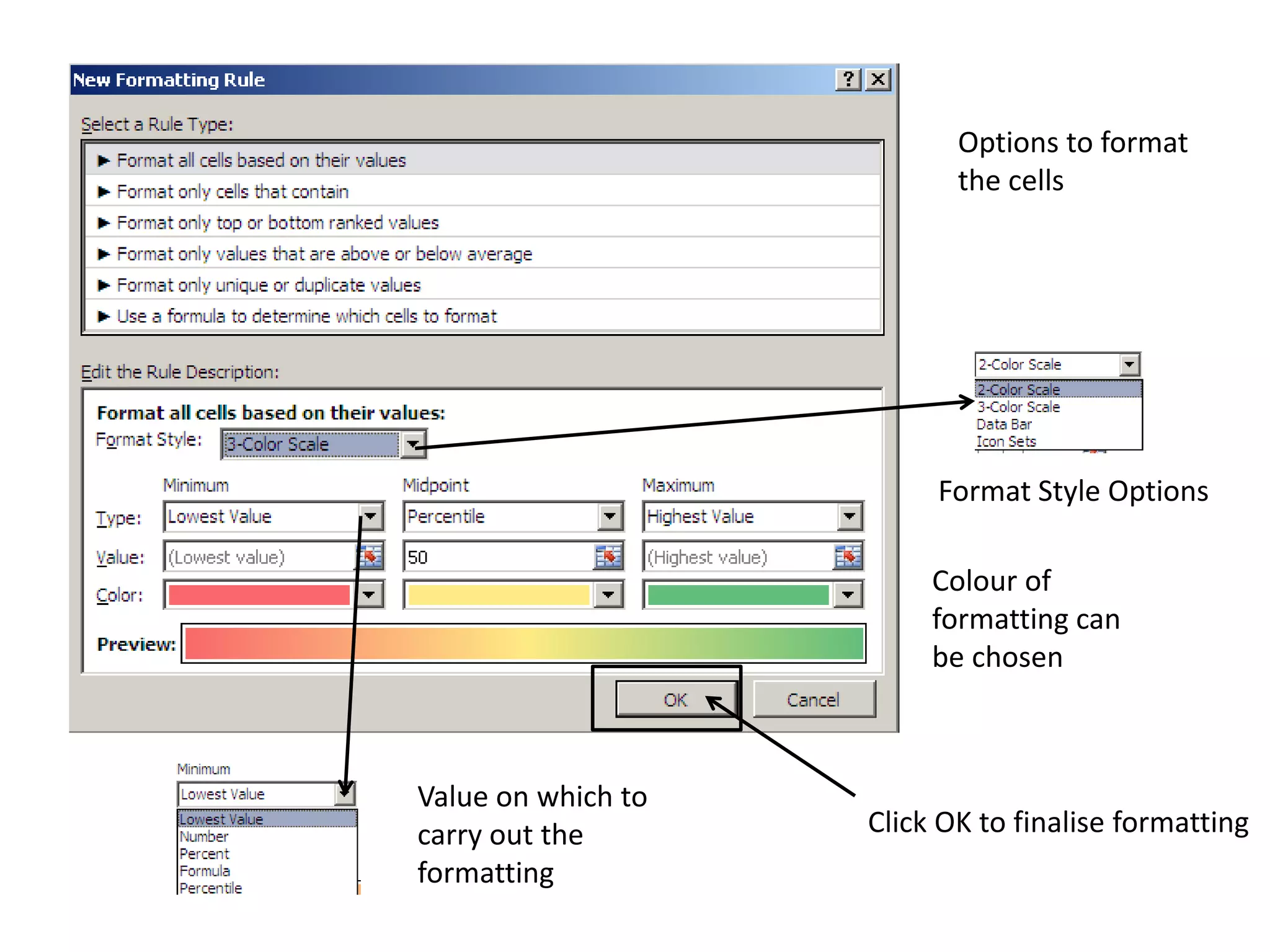
Instructions on applying Colour Scales for data visualization based on cell values for better analysis.
Steps to clear Conditional Formatting rules from the entire sheet, restoring the default format.