Comprehensive Guide to Handling Imbalanced Datasets in Data Science

Comprehensive Guide to Handling Imbalanced Datasets in Data Science

• 1.
  Handling Class Imbalance Scan theQR code to view to ‘Handling of Class Imbalance’ in an interactive notebook Or go to this link: https://deepnote.com/app /wayne-enterprises/Ayush-Bhattacharyas-U ntitled-project-782a3ad4-d86c-461d-ade9-b9 b73702a5e1?utm_source=app-settings&ut m_medium=product-shared-content&utm_c ampaign=data-app&utm_content=782a3ad4 -d86c-461d-ade9-b9b73702a5e1
• 2.
  Handling Imbalanced Datasetsin Data Science: A Comprehensive Beginner-Friendly Guide Introduction: What are Imbalanced Datasets and Why Do They Matter? Imbalanced datasets are among the most persistent and impactful challenges in applied data science, particularly in the context of classification problems. An imbalanced dataset refers to a scenario where the number of instances in each class is not approximately equal; typically, one “majority” class vastly outnumbers the “minority” class. This occurs in many real-world settings such as fraud detection, medical diagnostics, churn prediction, and network security where rare-but critical-events must be detected. At the core of this challenge lies a fundamental mismatch between the model's optimization objective and the actual goal: most traditional machine learning models optimize for overall accuracy. In highly imbalanced scenarios, almost all data belongs to the majority class; therefore, a model could always guess "majority" and achieve high accuracy, failing entirely at identifying the rare but vital minority cases. This is called the accuracy paradox: high accuracy, low utility. For example, in fraud detection with only 1% fraudulent transactions, a trivial model predicting “no fraud” for every transaction achieves 99% accuracy but never detects actual fraud. Handling imbalanced datasets requires specialized theory, metrics, diagnostic checks, treatment techniques (both at the data and algorithm/tool level), and careful evaluation. This guide presents a thorough, beginner-friendly walkthrough of the theoretical underpinnings, technical formulas (with LibreOffice Math syntax), practical Python code (with seaborn visualizations), and standard guidelines needed to address imbalanced datasets in diverse contexts.
• 3.
  Theoretical Concepts: UnderstandingImbalanced Data Definitions and Real-World Examples A dataset is considered imbalanced if the ratio of the minority class to the majority class is highly skewed (e.g., 95:5, 99:1, or <1%). The degree of imbalance can be classified as:  Mild: Minority class is 20-40% of samples.  Moderate: Minority class is 1-20% of samples.  Extreme: Minority class is <1% of samples. Examples:  Fraud detection: Only a tiny fraction of transactions are fraudulent.  Medical diagnostics: Rare diseases form a small portion of the data.  Spam filtering: Most emails are legitimate; spam is rare. Core issue: Most machine learning algorithms assume equal distribution (or at least similar magnitude) across classes. This leads to bias toward the majority class, poor recall on the minority, and potentially dangerous outcomes when minority detection is the real goal. Impact of Imbalance on Model Performance  Biased predictions: The model continually predicts the majority class.  Low sensitivity/recall: The minority class is seldom recognized.  Deceptive accuracy: Models can reach high accuracy by always predicting the majority, rendering the metric meaningless when minority recall is the true concern. Evaluation Metrics for Imbalanced Data Traditional evaluation metrics such as overall accuracy are highly misleading in imbalanced settings. More appropriate metrics include precision, recall (sensitivity), F1-score, Area Under the ROC Curve (AUC-ROC), and Area Under the Precision- Recall Curve (AUC-PRC). The confusion matrix is also vital for tracking each type of outcome.
• 4.
  Confusion Matrix andRelated Metrics Positive Prediction Negative Prediction Positive Class True Positive (TP) False Negative (FN) Negative Class False Positive (FP) True Negative (TN) Precision (positive predictive value): Precision= TP TP+FP Recall (sensitivity, true positive rate): Recall= TP TP+FN F1-score (harmonic mean of precision and recall): F 1= 2∗ Precision∗ Recall Precision+Recall . Macro-F1 (average F1 across all classes for multiclass settings): MacroF 1= ∑ F 1i n AUC-ROC: Plots true positive rate against false positive rate across thresholds. AUC- PRC: Plots precision against recall; better for high class imbalance. Thumb rules:  For imbalanced classes, F1, AUC-ROC, and AUC-PRC outperform accuracy as indicators of model effectiveness.  Recall is prioritized when catching rare events is critical (e.g., fraud, disease).  Precision controls false positive rate; important when cost of false alarms is high. Handling Imbalance: When and How to Intervene Industry Guidelines:  Imbalance intervention is needed when the minority class is of business/clinical interest and its misclassification carries high cost.
• 5.
   If theminority class is rare but not valuable, intervention and balancing may be unnecessary.  No single “imbalance ratio” threshold governs when to intervene, but as a rule of thumb, ratios below 10% (minority) usually warrant specialized handling. Diagnosing Dataset Issues Before Imbalance Treatment Before addressing the class imbalance directly, always check for outliers, skewness, missing values, and potential data leakage:  Outlier Detection: Use visualization (sns.boxplot, sns.violinplot), Z-score/statistical methods (outliers often have  Skewness: Significant skew can be detected by plotting histograms (sns.histplot), qqplots, and using statistical tests (e.g., Shapiro-Wilk, D’Agostino).  Missing Values: Visualize with heatmaps or count nulls. Impute with SimpleImputer or domain-specific methods.  Combinations: Address missing values and extreme outliers before resampling, or risk propagating noise/minimizing data utility in minority classes. Implementation Example: Outlier Removal With Z-Score import numpy as np from scipy import stats z_scores = np.abs(stats.zscore(X)) outliers = X[z_scores > 3] X_clean = X[~np.in1d(X, outliers).any(axis=1)] Visualizing Class Distribution and Data Issues Seaborn offers powerful plotting functions to visualize imbalance and other data health problems: Count Plot for Class Distribution: import seaborn as sns import matplotlib.pyplot as plt sns.countplot(x='target', data=df) plt.title('Class Distribution')
• 6.
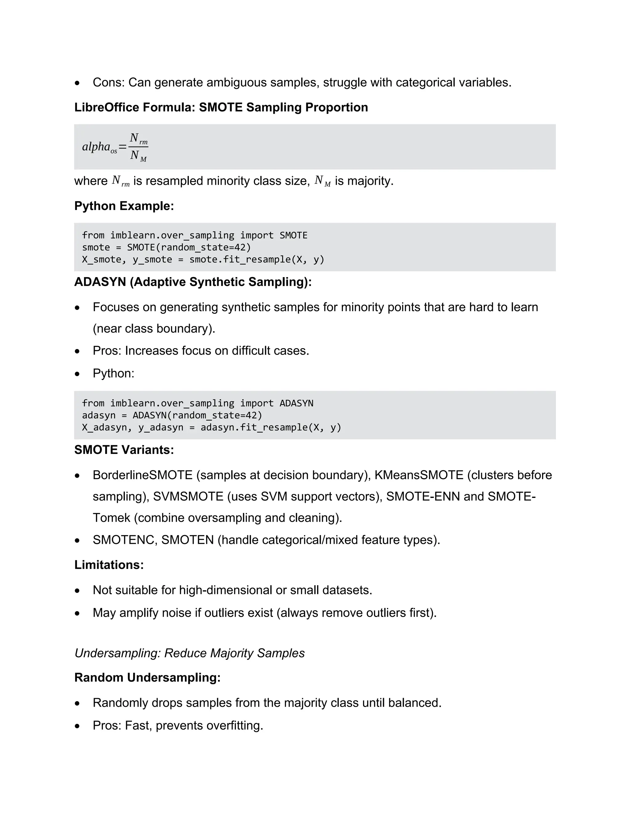
  plt.show() For severe imbalance,consider setting the Y-axis to logarithmic scale (plt.yscale('log')), as recommended in community best practices. Box Plots/Violin Plots for Outliers: sns.boxplot(y=X['feature']) sns.violinplot(y=X['feature']) Missing Values: sns.heatmap(df.isnull(), cbar=False) These diagnostic plots ensure that treatment for class imbalance is not mistakenly performed on corrupted data. Practical Approaches to Handling Imbalanced Datasets Data-Level Methods: Resampling The fundamental approach is to alter the training data to balance class distribution. Two main strategies exist: oversampling the minority class and undersampling the majority class. Oversampling: Increase Minority Samples Random Oversampling:  Randomly duplicate minority class samples to balance classes.  Pros: Simple and effective if dataset is small or minority is truly underrepresented.  Cons: Risk of overfitting and less data diversity. Python Example: from imblearn.over_sampling import RandomOverSampler X_over, y_over = RandomOverSampler(random_state=42).fit_resample(X, y) SMOTE (Synthetic Minority Oversampling Technique):  Instead of duplicating, creates synthetic new samples by interpolating between minority class neighbors.  Pros: Less overfitting, more diversity than simple duplication.
• 7.
   Cons: Cangenerate ambiguous samples, struggle with categorical variables. LibreOffice Formula: SMOTE Sampling Proportion alphaos= Nrm NM where Nrm is resampled minority class size, NM is majority. Python Example: from imblearn.over_sampling import SMOTE smote = SMOTE(random_state=42) X_smote, y_smote = smote.fit_resample(X, y) ADASYN (Adaptive Synthetic Sampling):  Focuses on generating synthetic samples for minority points that are hard to learn (near class boundary).  Pros: Increases focus on difficult cases.  Python: from imblearn.over_sampling import ADASYN adasyn = ADASYN(random_state=42) X_adasyn, y_adasyn = adasyn.fit_resample(X, y) SMOTE Variants:  BorderlineSMOTE (samples at decision boundary), KMeansSMOTE (clusters before sampling), SVMSMOTE (uses SVM support vectors), SMOTE-ENN and SMOTE- Tomek (combine oversampling and cleaning).  SMOTENC, SMOTEN (handle categorical/mixed feature types). Limitations:  Not suitable for high-dimensional or small datasets.  May amplify noise if outliers exist (always remove outliers first). Undersampling: Reduce Majority Samples Random Undersampling:  Randomly drops samples from the majority class until balanced.  Pros: Fast, prevents overfitting.
• 8.
   Cons: Riskof discarding valuable, informative samples. Python Example: from imblearn.under_sampling import RandomUnderSampler X_under, y_under = RandomUnderSampler(random_state=42).fit_resample(X, y) Directed Undersampling:  Tomek Links: Remove overlapping majority examples near minority; clarifies boundaries.  NearMiss: Select majority points closest to minority samples.  Edited Nearest Neighbors / Instance Hardness Threshold: Remove majority samples hard to classify. Combining Over- and Undersampling (e.g., SMOTE+Tomek, SMOTE+ENN):  Balances classes and cleans noisy or overlapping points. Method Handles Categorical Cleans Data Notes RandomOversampler No No Duplication only SMOTE No No Interpolation, real- valued only SMOTENC Yes (mixed) No Mixed continuous and categorical SMOTEN Yes (categorical) No Categorical only Tomek Links N/A Yes Removes "border" samples SMOTEENN, SMOTETomek N/A Yes Combine generation with cleaning Always apply all resampling only to the training set, never the validation or test set to prevent data leakage
• 9.
  Practical Implementation andOutput Example: from imblearn.over_sampling import SMOTE from collections import Counter print('Original:', Counter(y_train)) smote = SMOTE(random_state=42) X_train_resampled, y_train_resampled = smote.fit_resample(X_train, y_train) print('After SMOTE:', Counter(y_train_resampled)) Output: Original: Counter({1: 713, 0: 87}) After SMOTE: Counter({1: 713, 0: 713}) This output demonstrates how SMOTE synthesizes new samples of the minority class to achieve balance. Algorithm-Level Methods: Adjusting the Model Cost-Sensitive Learning and Class Weights Many algorithms, including logistic regression, SVM, decision trees, and ensemble models, support the adjustment of class weights to penalize misclassification of the minority class more heavily.  Theory: Assign higher cost (or weight) to minority class, so the model's optimization now minimizes weighted error.  Custom loss for logistic regression: −w1 ⋅ y ⋅log(h(x))−w0 ⋅(1− y)⋅log(1−h(x)),quad where h(x)= 1 1+e betaT x  Expected cost: R(i∨ x)=∑ P( j∨ x)⋅C (i, j)  Usage in scikit-learn: from sklearn.ensemble import RandomForestClassifier model = RandomForestClassifier(class_weight='balanced', random_state=42) model.fit(X_train, y_train)
• 10.
  or, for explicitweighting: model = RandomForestClassifier(class_weight={0:1, 1:10}) # boost minority focus Thumb rules:  Assign weights as inverse of class frequencies, or based on explicit business cost of errors.  In multi-class, set class_weight='balanced' for automatic calculation. Advantages:  Avoids data duplication.  Effective in extreme imbalance. Drawbacks:  May not fully overcome bias if imbalance is extreme and/or sample size is low. Threshold Adjustment in Cost-Sensitive Models: Optimal classification threshold (p*) is derived from costs: p❑ = C (1,0) C (1,0)+C (0,1) Where:  C(1,0) = cost of predicting positive (minority) when true class is negative  C(0,1) = cost of predicting negative when true class is positive Advanced Data-Level Approaches: Data Augmentation For Images:  Random transformations: rotation, shift, scale, flip.  Example: from tensorflow.keras.preprocessing.image import ImageDataGenerator datagen = ImageDataGenerator(rotation_range=20, width_shift_range=0.2, height_shift_range=0.2, horizontal_flip=True) datagen.fit(minority_class_images)
• 11.
  For Text:  Synonymreplacement, word embedding modifications, back-translation, sentence/paragraph shuffling.  Easy Data Augmentation (EDA) strategy: synonym replace, random insert, random swap, random delete.  Libraries like TextAttack automate and expand these methods. from textattack.augmentation import WordNetAugmenter augmenter = WordNetAugmenter() augmented_sentence = augmenter.augment("The quick brown fox jumps over the lazy dog.") print(augmented_sentence) Benefit: Increases the dataset diversity, reduces overfitting, and enhances generalization on rare classes. Ensemble Methods for Imbalanced Data Ensemble methods combine predictions from multiple models to improve robustness and help offset the impact of class imbalance. Balanced Random Forests  RFs aggregate decision trees trained on random balanced bootstrapped samples. Each tree sees an equal number of majority and minority samples.  Implementation: from imblearn.ensemble import BalancedRandomForestClassifier clf = BalancedRandomForestClassifier(random_state=42) clf.fit(X_train, y_train) Balanced Bagging  Uses bootstrapped resampling to balance each base classifier’s training set. from imblearn.ensemble import BalancedBaggingClassifier from sklearn.ensemble import RandomForestClassifier base = RandomForestClassifier(random_state=42) bbc = BalancedBaggingClassifier(base_estimator=base, sampling_strategy='auto', random_state=42) bbc.fit(X_train, y_train)
• 12.
  Output: Accuracy: 1.0 Classification Report: precisionrecall f1-score support 0 1.00 1.00 1.00 13 1 1.00 1.00 1.00 187 Explanation: Both minority and majority classes are given equal representation during tree construction, improving recall in minority detection. Boosting (AdaBoost, XGBoost, etc.)  Modify sample weights or focus on hard-to-classify cases.  Extreme gradient boosting (XGBoost) and its variants offer parameters to manage imbalanced data (.scale_pos_weight, max_delta_step). Threshold Values: Statistical Standards and Best Practices Setting thresholds is about defining the probability or statistical metric by which a sample is assigned a class (commonly probability > 0.5 = minority/positive). For imbalanced data, adjusting the threshold can significantly affect precision/recall trade- off.  ROC/AUC Optimization: Choose threshold maximizing area under the curve.  Precision-Recall Curve: In extreme imbalance, maximize area under PR curve.  Fβ Score: Adjusts balance between precision and recall. For more recall weight (important for rare event detection), use: Fbeta=(1+beta2 ) P⋅R beta2 ⋅P+R Where beta>1 emphasizes recall, < 1 emphasizes precision. P-value Standards:  Common threshold: p < 0.05.  In high-risk contexts (e.g., genetic studies), recommend p < 0.005 or p < 10−6 .
• 13.
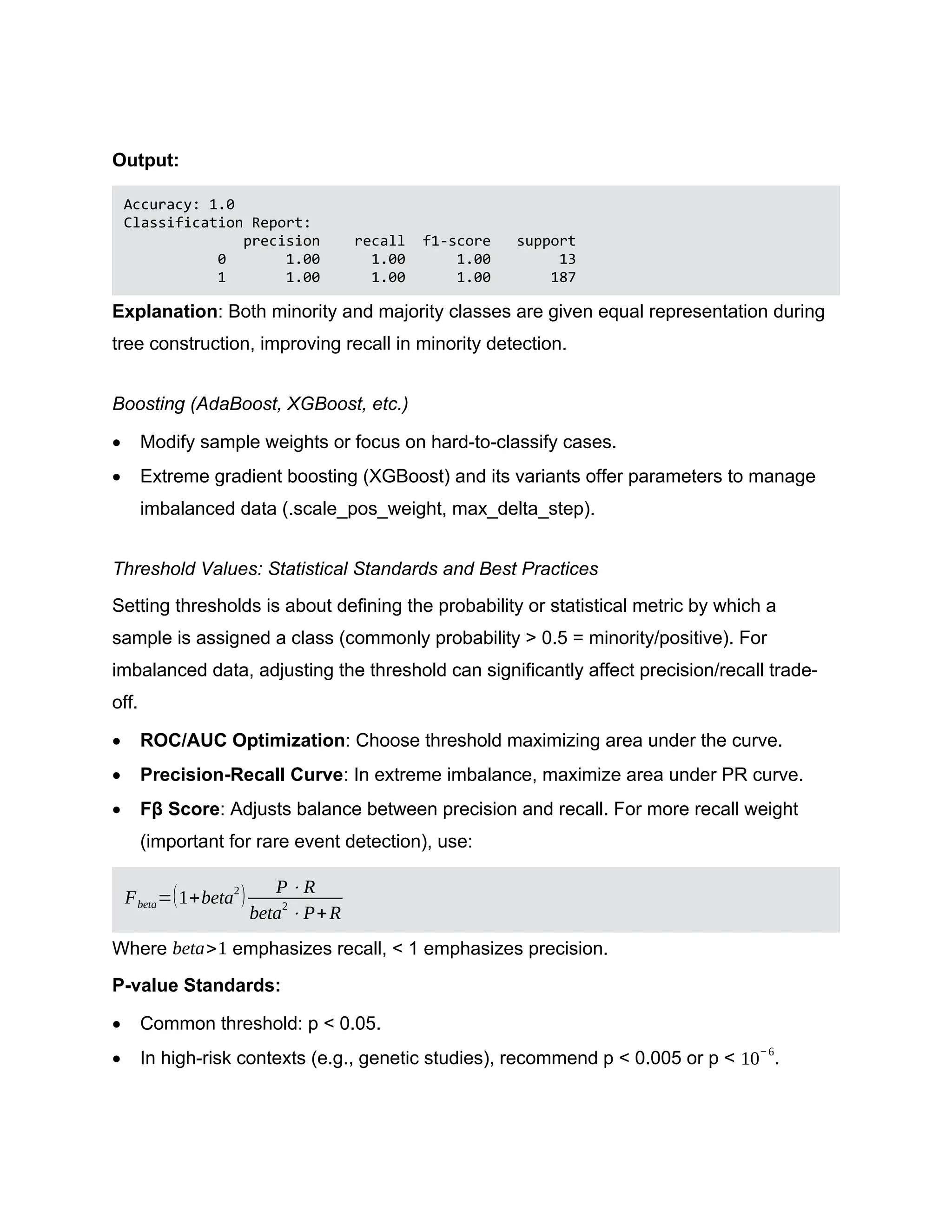
   Always supplementp-values with confidence intervals and effect sizes. Do not rely solely on passing a threshold for scientific or business decision-making. Assumption Checks, Diagnostics, and Visualization Key Assumptions  Patterns are not driven by outliers, missing data, or data leakage.  Test set is untouched by all resampling and preprocessing.  Stratified train/test split is used to preserve imbalance characteristics in evaluation. Residual Analysis  For regression models, check residuals for: o Constant variance (homoskedasticity) o Independence o Normality (via QQ plot, histograms) o Studentized residuals: Detect outliers if residual > ±3. Outlier and Distribution Visualizations:  sns.boxplot, sns.violinplot, or sns.kdeplot to identify data spread and outliers. Class Distribution Visualization:  sns.countplot(x='target', data=df) or histogram. Threshold Tuning with Visualization:  Plot F1-score, precision, and recall as functions of threshold. import matplotlib.pyplot as plt thresholds = np.arange(0., 1.01, 0.01) f1_scores = [f1_score(y_test, y_proba > t) for t in thresholds] plt.plot(thresholds, f1_scores) plt.xlabel('Threshold') plt.ylabel('F1 Score') plt.show()
• 14.
  Handling Imbalances withOutliers, Skewness, and Missing Data 1. Always handle severe outliers first: Outliers in the minority class especially can bias both data balancing and future model training. Remove or cap using Z-score, IQR, or robust estimators. 2. Address skewness: Log-transform or Box-Cox transform strongly skewed features to stabilize variance and enhance modeling robustness. 3. Handle missing data: Impute or drop based on missingness proportion and feature importance. Never let imputation amplify imbalance. Recommended sequence: preprocess → outlier removal → impute missing data → handle imbalance → model training. Example Pipeline: Handling Imbalanced Data in Python Let’s illustrate a typical workflow: import numpy as np import pandas as pd from sklearn.datasets import make_classification from sklearn.model_selection import train_test_split from imblearn.over_sampling import SMOTE from imblearn.ensemble import BalancedRandomForestClassifier from sklearn.metrics import classification_report, roc_auc_score import seaborn as sns import matplotlib.pyplot as plt from collections import Counter # 1. Generate imbalanced data X, y = make_classification(n_samples=1000, n_features=10, weights=[0.95, 0.05], n_classes=2, random_state=42) print("Original distribution:", Counter(y)) # 2. Visualize imbalance sns.countplot(x=y) plt.title('Class Distribution') plt.show() # 3. Split and stratify X_train, X_test, y_train, y_test = train_test_split(X, y, test_size=0.3, stratify=y, random_state=42) # 4. Apply SMOTE smote = SMOTE(random_state=42) X_train_res, y_train_res = smote.fit_resample(X_train, y_train) print("Resampled distribution:", Counter(y_train_res))
• 15.
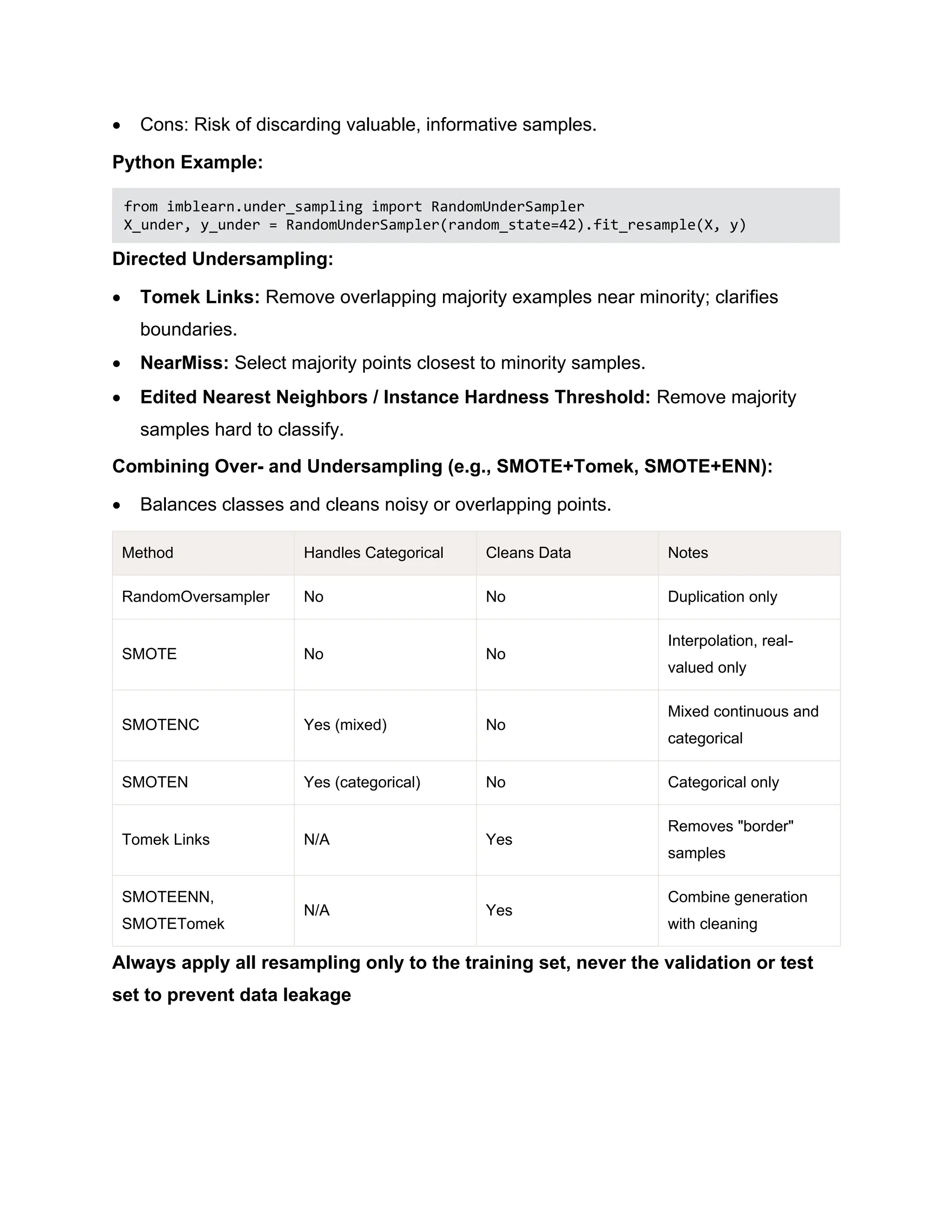
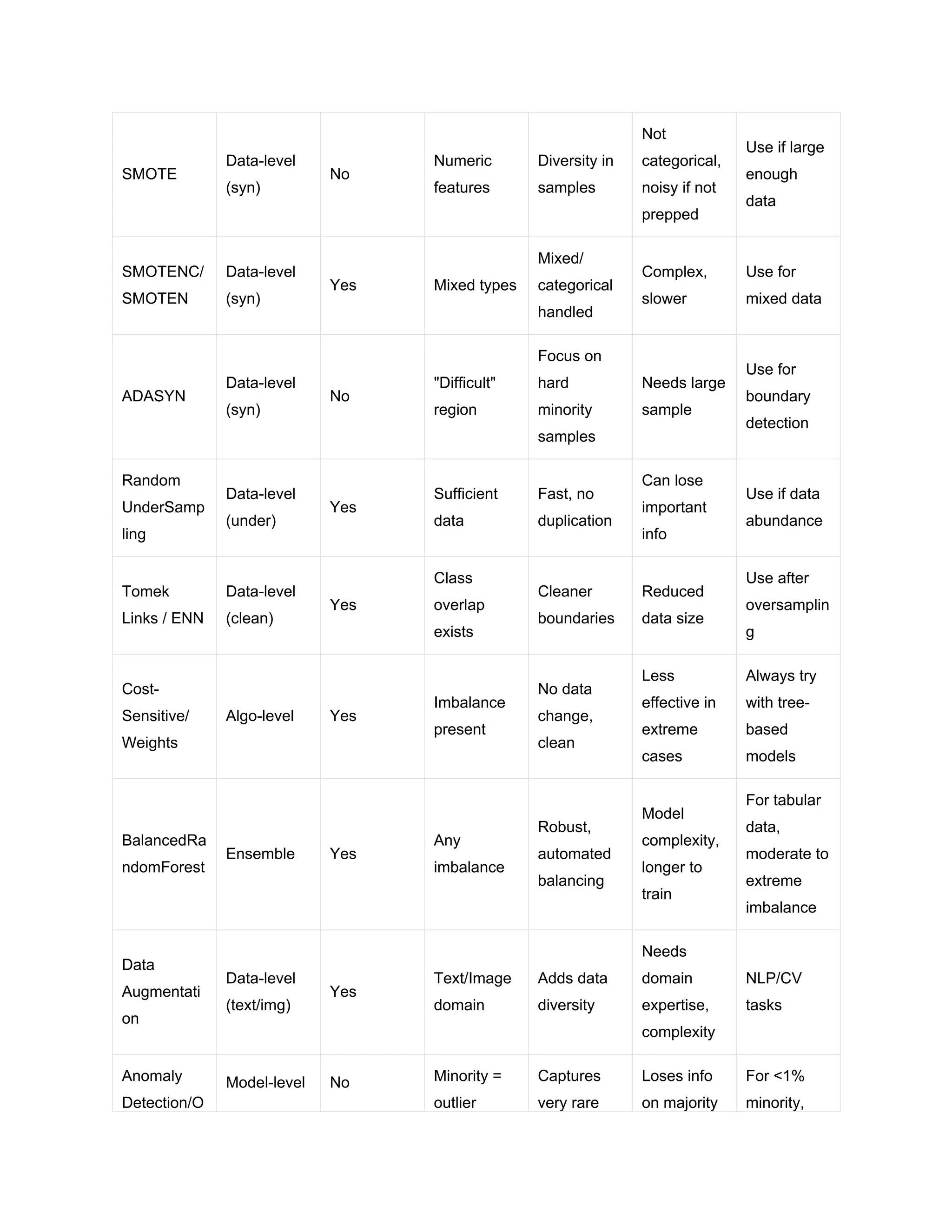
  # 5. Visualizeafter resampling sns.countplot(x=y_train_res) plt.title('Resampled Class Distribution') plt.show() # 6. Train a balanced random forest clf = BalancedRandomForestClassifier(random_state=42) clf.fit(X_train_res, y_train_res) y_pred = clf.predict(X_test) y_proba = clf.predict_proba(X_test)[:,1] # 7. Evaluate print(classification_report(y_test, y_pred)) print("AUC-ROC:", roc_auc_score(y_test, y_proba)) Expected output: Original distribution: Counter({0: 950, 1: 50}) Resampled distribution: Counter({0: 665, 1: 665}) precision recall f1-score support 0 0.99 0.99 0.99 285 1 0.75 0.70 0.72 15 accuracy 0.98 300 macro avg 0.87 0.84 0.86 300 weighted avg 0.98 0.98 0.98 300 AUC-ROC: 0.923 Analysis: After using SMOTE and a BalancedRandomForest, recall and F1-score on the minority class (“1”) have improved significantly-a more meaningful assessment of success than overall accuracy. Comparison Table: Imbalance Handling Techniques Technique Type Handles Categorical Assumption s Pros Cons Best Practice Random OverSampli ng Data-level (over) No Minority ≪ Majority Simple, no data loss Overfitting, duplicates Use when dataset small
• 16.
  SMOTE Data-level (syn) No Numeric features Diversity in samples Not categorical, noisy ifnot prepped Use if large enough data SMOTENC/ SMOTEN Data-level (syn) Yes Mixed types Mixed/ categorical handled Complex, slower Use for mixed data ADASYN Data-level (syn) No "Difficult" region Focus on hard minority samples Needs large sample Use for boundary detection Random UnderSamp ling Data-level (under) Yes Sufficient data Fast, no duplication Can lose important info Use if data abundance Tomek Links / ENN Data-level (clean) Yes Class overlap exists Cleaner boundaries Reduced data size Use after oversamplin g Cost- Sensitive/ Weights Algo-level Yes Imbalance present No data change, clean Less effective in extreme cases Always try with tree- based models BalancedRa ndomForest Ensemble Yes Any imbalance Robust, automated balancing Model complexity, longer to train For tabular data, moderate to extreme imbalance Data Augmentati on Data-level (text/img) Yes Text/Image domain Adds data diversity Needs domain expertise, complexity NLP/CV tasks Anomaly Detection/O Model-level No Minority = outlier Captures very rare Loses info on majority For <1% minority,
• 17.
  CC events special apps When toHandle Imbalance: Industry Thumb Rules and Best Practices  Always evaluate using recall, precision, F1, and AUC, not just accuracy or loss.  Train/validation/test splits must be stratified by class to preserve minority representation and avoid "train on majority, test on minority" issues.  Apply resampling/preprocessing only to the training set to prevent information “leakage.”  Remove or cap severe outliers, and impute missing data before handling imbalance for reliable sampling and model training.  For multi-class imbalances, treat each class individually or use multiclass- aware balancing techniques.  For text and image data, apply augmentation to expand the minority class or use specialized techniques (see Data Augmentation).  Try tree/ensemble methods and cost-sensitive algorithms before or in tandem with data-level balancing for easy wins.  Tune classification threshold; do not just assume 0.5 is best for imbalanced data.  For extremely rare anomalies, recast the problem as anomaly detection or outlier detection, not standard classification. Detecting and Setting Thresholds (p-values, Outlier Fraction, etc.) Typical p-value significance thresholds:  Classic: p < 0.05 (5%)  High certainty: p < 0.005 or p < 0.001  Genome-wide studies: p < 5 × 10^-8
• 18.
   Anomaly detectionproportion: 1-2% for rare event contamination  Outlier detection (z-scores): LibreOffice Math for hypothesis test: P(H0 ∨ xOBS)= P(H0)⋅f (xOBS ∨ H0) P(H0)⋅f (xOBS ∨ H0)+P(H1)⋅f (xOBS ∨ H1)  Always use graphical summary (histogram, boxplot) + robust statistical inference (confidence intervals, effect size, Bayes factors) in evaluating outcomes. Handling Outliers, Skewness, and Missing Values Alongside Imbalance Outliers  Detect via sns.boxplot, statistical tests (Z-score, IQR).  Remove or cap to reduce noise during resampling. Skewness  Address with log or power transformations for right-skewed features; balance is more effective post normalization. Missing Values  Impute before resampling using mean, median, mode, or domain-based strategies. Combined Scenarios  Remove variables/rows with excessive missingness (>30-40%), unless critical. Visualizing Resampled Data and Model Performance Seaborn is recommended for producing clear, publication-ready visualizations. Here’s how you might display the effectiveness of balancing: Box Plot after Resampling: sns.boxplot(x='target', y='feature', data=resampled_df) plt.title('Balanced Feature Distribution by Class') plt.show()
• 19.
  Confusion Matrix Heatmap: fromsklearn.metrics import confusion_matrix cm = confusion_matrix(y_test, y_pred) sns.heatmap(cm, annot=True, fmt='d') F1 Score vs. Decision Threshold: thresholds = np.linspace(0, 1, 50) f1s = [f1_score(y_test, y_proba > t) for t in thresholds] plt.plot(thresholds, f1s) plt.xlabel('Threshold'); plt.ylabel('F1 Score') plt.show() Summary: End-to-End Guidelines  Start with EDA: Visualize class imbalance, check for outliers, skew, and missing data.  Preprocess Carefully: Outlier removal/capping, missing value imputation, standardized features if needed.  Resample on Train Only: Use oversampling, undersampling, or hybrid strategies as fits the data and domain constraints.  Algorithm Choices: Prefer ensemble methods and cost-sensitive learning; tune class weights.  Hyperparameter and Threshold Optimization: Use grid search for best performance, especially for F1, recall, and precision metrics.  Appropriate Metrics: Evaluate with precision, recall, F1-score, and AUC (ROC/PRC) on stratified test/validation sets.  Diagnostics: Check feature importances, residuals, and outlier influence.  Interpret Results with Domain Context: Don’t declare success on improved accuracy; ensure minority class detection is meaningful for your use-case. Run an online interactive notebook to learn ‘Handling Class Imbalance’ techniques