Comparative Study of Object Detection Algorithms

Comparative Study of Object Detection Algorithms

• 1.
  International Research Journalof Engineering and Technology (IRJET) e-ISSN: 2395-0056 Volume: 04 Issue: 11 | Nov -2017 www.irjet.net p-ISSN: 2395-0072 Comparative Study of Object Detection Algorithms Nikhil Yadav1 , Utkarsh Binay2 1Student,Computer Engineering Department, Rizvi College of Engineering, Maharashtra, India 2Student, Computer Science Department, Mukesh Patel School of Technology And Management, Maharashtra, India ---------------------------------------------------------------------***--------------------------------------------------------------------- Abstract - This paper aims to find the best possible combination of speed and accuracy while comparing different object detection algorithms that use convolutional neural networks to perform object detection. Models which are usually computationally expensive, achieve the best accuracy, but cannot be deployed in a simple setting with limited resources, whereas, faster models fail to achieve similar results compared to their bigger and more memory intensive counterparts. We discuss two ends of a spectrum here comparing three different models ,i.e Single Shot Detector (SSD) [1], Faster R-CNN (Region - based Convolutional Neural Networks)[3], R-FCN(Region based-Fully Convolutional Networks)[2], where on one end we get a model which can be deployed on a mobile device because of its speed and another model which is at the cutting edge of performance when it comes to accuracy. These models are trained and their performance metrics tested on the COCO ( common objects in context) dataset. Key Words: COCO dataset, Bounding boxes, Single Shot Detector, Inception Resnet, Resnet-101, Mobile Net, VGG- 16(Visual Geometry Group),Faster R-CNN, R-FCN, Hyper parameter tuning, mAP( mean average precision) 1.INTRODUCTION State of the art computer vision systems have involved a range of object detection models that use convolutional neural networks in their working. The deployment of these models like YOLO[9], SSD[1], R-FCN[2],R-CNN, etc depends on the kind of usage we want. Google photos has deployed models like SSD Mobile Net which is known for its speed and isn’t memory intensive, here performance isn’t the most important factor ,but memory efficiency is. In case of self driving cars though, the requirement for an extremely accurate model is a priority, as these real time systems are performing tasks which can lead to a life and death situation in their surrounding. We need to evaluate these models using several evaluation metrics like mAP, memory requirement ,testing time. We have only considered models which are quite similar in their architecture on a high level overview. The models that are considered are Faster R-CNN[3], R-FCN[2], SSD[1] , these models have used sliding window style predictions and have only used a single CNN network. These models are responsible for the object detection part, whereas the feature extraction part is carried out by the different image classification models , the state of the art ones which have participated in the image net competitions. We refer to the object detection models as meta architectures and they are coupled with different feature extractors for eg( VGG, Resnet, Mobile Net[10]), to evaluate the various combinations we get through them. We would first describe the different meta architectures and then the different feature extractors, and then compare their combinations by testing them on the objects present in the COCO dataset. In this paper we have tried to perform this experiment in controlled conditions with same hardware conditions for comparison and run these tests multiple times so that they prove to be statistically consistent. We have used the deep learning library Tensorflow[5] for our implementation. Previous experiments by others have been performed on caffe, and tried on other standard datasets like PASCAL VOC(Visual Object Classes). A few have fine tuned the detectors for their specific objects and noted the test times for different models. The main reason for using tensor flow[5] was its portability and ease of use. Fig-1: An example of an object detector in use 2. META ARCHITECTURE Modern meta architectures all use CNN for object detection , let us have a look at the history of a few meta architectures that we are discussing, and have an in depth look at their inner working. © 2017, IRJET | Impact Factor value: 6.171 | ISO 9001:2008 Certified Journal | Page 586
• 2.
  International Research Journalof Engineering and Technology (IRJET) e-ISSN: 2395-0056 Volume: 04 Issue: 11 | Nov -2017 www.irjet.net p-ISSN: 2395-0072 2.1 R-CNN The R-CNN model was one of the first models to use convolutional neural networks for object detection. The goal of R-CNN is to take in an image, and correctly identify where the main objects (via a bounding box) in the image. But how do we find out where these bounding boxes are? R-CNN does what we might intuitively do as well -propose a bunch of boxes in the image and see if any of them actually correspond to an object. R-CNN creates these bounding boxes, or region proposals using a process called Selective Search. Selective search, looks at the image through windows of different sizes, and for each size tries to group together adjacent pixels by texture, color, or intensity to identify objects. Once the proposals are created, R-CNN warps the region to a standard square size and passes it through to a feature extractor or image classifier , which is a CNN. On the final layer of the CNN, R- CNN adds a Support Vector Machine (SVM) that simply classifies whether this is an object, and if yes, which object is it. 2.2 Fast R-CNN R-CNN works really well, but is really quite slow for a few simple reasons It requires a forward pass of the CNN for every single region proposal for every single image. It has to train three different models separately - the CNN to generate image features, the classifier that predicts the class, and the regression model to tighten the bounding boxes. This makes the pipeline extremely hard to train. Both these problems were solved in Fast R-CNN[4] by the creator of R-CNN himself. For the forward pass of the CNN, Girshick realized that for each image, a lot of proposed regions for the image invariably overlapped causing us to run the same CNN computation again and again . His insight was simple — Why not run the CNN just once per image and then find a way to share that computation across the proposals? .This is exactly what Fast R-CNN does using a technique known as RoI Pool (Region of Interest Pooling). At its core, RoI Pool shares the forward pass of a CNN for an image across its subregions. In the image above, notice how the CNN features for each region are obtained by selecting a corresponding region from the CNN’s feature map. Then, the features in each region are pooled (usually using max pooling). So all it takes us is one pass of the original image .The second insight of Fast R- CNN is to jointly train the CNN, classifier, and bounding box regressor in a single model. Where earlier we had different models to extract image features (CNN), classify (SVM), and tighten bounding boxes (regressor),Fast R- CNN[4] instead used a single network to compute all three. Fast R-CNN replaced the SVM classifier with a softmax layer on top of the CNN to output a classification. It also added a linear regression layer parallel to the softmax layer to output bounding box coordinates. In this way, all the outputs needed came from one single network. 2.3 Faster R-CNN There was still one bottleneck with Fast R-CNN which had to be sorted, that was the region proposer. The very first step to detecting the locations of objects is generating a bunch of potential bounding boxes or regions of interest to test. In Fast R-CNN, these proposals were created using Selective Search, a fairly slow process that was found to be the bottleneck of the overall process. Faster R-CNN[3] found a way a to make the step of region proposal almost cost free. The insight of Faster R-CNN was that region proposals depended on features of the image that were already calculated with the forward pass of the CNN (first step of classification). So why not reuse those same CNN results for region proposals instead of running a separate selective search algorithm? Indeed, this is just what the Faster R-CNN team achieved. In this model, a single CNN is used to both carry out region proposals and classification. This way,only one CNN needs to be trained and we get region proposals almost for free. How the Regions are Generated? Let’s take a moment to see how Faster R-CNN generates these region proposals from CNN features. Faster R-CNN adds a Fully Convolutional Network on top of the features of the CNN creating what’s known as the Region Proposal Network. Fig-2 : The Region Proposal Network slides a window over the features of the CNN. At each window location, the network outputs a score and a bounding box per anchor (hence 4k box coordinates where k is the number of anchors) 2.4 R-FCN With the increase in performance, Faster R-CNN was an order of magnitude swifter than its earlier counterpart fast R-CNN .But there was issue of applying the region- specific component had to be applied several times in an image, this issue was resolved in R-FCN (Region based Fully Convolutional networks) where the computation required per image was reduced drastically, where instead of cropping features from the same layer where the crops are predicted, the crops are taken from last layer of features prior to predictions. The algorithm works faster than Faster R-CNN while achieving comparable accuracy © 2017, IRJET | Impact Factor value: 6.171 | ISO 9001:2008 Certified Journal | Page 587
• 3.
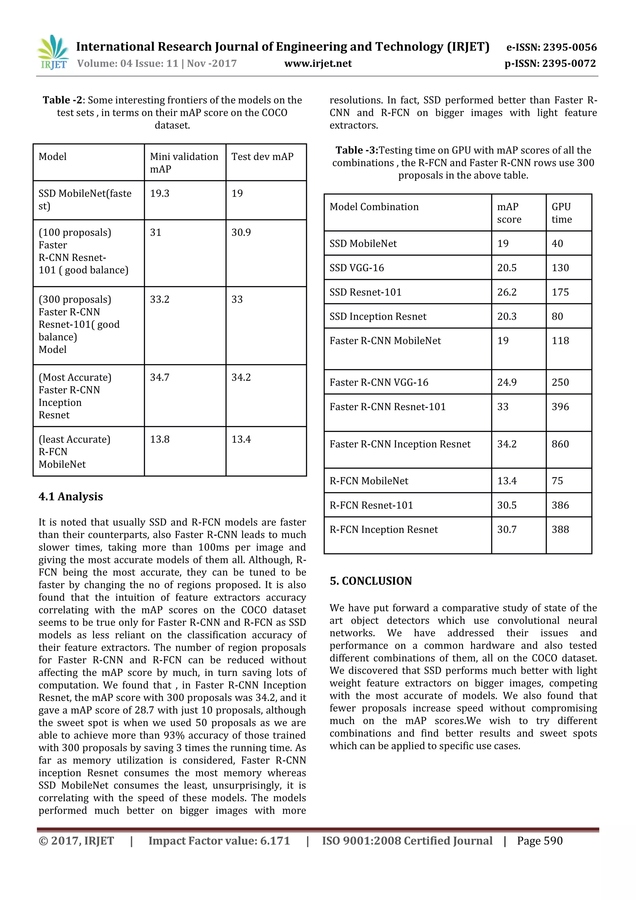
  International Research Journalof Engineering and Technology (IRJET) e-ISSN: 2395-0056 Volume: 04 Issue: 11 | Nov -2017 www.irjet.net p-ISSN: 2395-0072 scores when run using Resnet101 as the feature extractor, on the hindsight, it also respects translational invariance, as it is a position sensitive cropping mechanism. 2.5 SSD(Single Shot Detector) SSD works by converting discrete output spaces for bounding boxes into sets of default boxes for different aspect ratios and for every feature map location. During predictions, the model generates the scores in each default box for every object detected and scales the default box to fit the object shape. SSD is simpler than other networks as it performs all computations in a single network. SSD combines the predictions from numerous feature maps having different resolutions to handle objects of various sizes. It doesn’t involve regional proposal generating or feature resampling like previous networks did, which makes it easy to train and integrate into systems where detection is required. 3. EXPERIMENTAL SETUP 3.1 Feature Extractors We will be discussing a few feature extractors to get the gist of the entire architecture, where meta architectures are combined with feature extractors like VGG, Resnet101 etc. The way it works is that we first apply convolutional neural networks via feature extractors to extract all the high level information from the images. The feature extractors must be wisely selected as types of layers, no of parameters directly affect the speed and memory performance of the object detectors. We will compare four different feature extractors to combine with our meta architectures and test their performances. Out of the four chosen feature extractors , apart from Mobile Net, every other feature extractor has an open source Tensor flow implementation, which one can use via GitHub. We compare VGG-16, Resnet101, Inception Resnet(v2)[6] ,which combines the optimization quality of ResNet with computational efficiency of inception modules and Mobile Net which achieved accuracies similar to VGG-16 in Image net competition with 1/30 of its computational cost and model size. As the name suggests, Mobile Net because of its low computational cost has been at the forefront of various vision applications in mobile devices. Its building blocks are depth wise separable convolutions which factorize a standard convolution into a depth wise convolution and a 1x1 convolution, effectively reducing both computational cost and number of parameters. In R- FCN and R-CNN , where we must choose the layer that must be used for predicting region proposals, we have used ‘Conv5’ layer in VGG-16, and ‘Conv_4_x’ layers in ResNet-101, for other feature extractors we choose similar layers. In SSD, following previous methodologies, we have also selected the topmost convolutional feature map and a higher resolution feature map at a lower level, then adding a sequence of convolutional layers with spatial resolution decaying by a factor of 2 with each additional layer used for prediction. We have used batch normalization in all layers of the single shot detector. 3.2 Number Of Proposals The no of region proposals that can be sent across to the box classifier at test time can be varied. The default number is 300 but we have tried a range of numbers .It was noted that there was a trade-off between computation cost and recall, so there was a balance to be maintained. We have tried no of boxes ranging from 10 to 300 in our exploration. 3.3 Loss Function Configuration In our experiments we use Argmax matching throughout with thresholds set as suggested in the original paper for each meta-architecture. Also, using the ratios described in the original papers of each meta architecture , we have fixed the ratios of positive anchors and negative anchors. 3.4 Training and Hyperparameter Tuning For Faster R-CNN and R-FCN, we have used Stochastic gradient descent with momentum with batch size, as the image sizes used were different, so they were being trained independently, for SSD we have used 32 as the batch size as they were resized to a fixed shape. The learning rates were tuned manually for each feature extractor. The networks were trained on the COCO dataset ,where we held 7000 images for validation. The model was evaluated in the official COCO API where the mAP is measured. 3.5 Hardware We ran the experiment on a Nvidia Titan X GPU card ,on a 32 GB RAM device with Intel Xeon E5-1650 v2 processor. The images were resized and the dimensions were k x k, where k is either 300 or 600 . The timings were averaged for 450 images. 3.6 Model Details Here, we mention the intricate details of the different combination of meta architectures with the feature extractors. 3.6.1 Faster R-CNN Tensorflow’s “crop_and_resize” is used instead of standard ROI pooling, also batch normalization is used in all convolutional layers. Optimizer used is SGD with momentum set to 0.9. The learning rate was set as per the feature extractor. © 2017, IRJET | Impact Factor value: 6.171 | ISO 9001:2008 Certified Journal | Page 588
• 4.
  International Research Journalof Engineering and Technology (IRJET) e-ISSN: 2395-0056 Volume: 04 Issue: 11 | Nov -2017 www.irjet.net p-ISSN: 2395-0072 VGG-16: The initial learning rate is set to 5e-4,we extract features from the conv5 layers, we resize feature maps to 14x14 and maxpool layers of 7x7 is used . Resnet-101: The initial learning rate is set to 3e-4, we extract features from the final layer of conv4 block, stride size is of 16 pixels. Inception Resnet: The stride size is 8 in atrous mode, and 16 otherwise. The features are extracted from the Mixed_6a layers including the residual layers. Features maps are 17x17 size and learning rate is 1e-3. MobileNet: The initial learning rate is 3e-3 and stride size is set to 16 pixels. We extract features from Conv2D_11 layers and features maps of size 14x14 are used. 3.6.2 R-FCN The parameters set are identical to those of R-CNN with use of crop_and_resize, SGD with momentum 0.9, use of batch normalization,etc. R-FCN was trained using Resnet, Inception Resnet and MobileNet[10] feature extractors. Resnet 101: Features are extracted from block3 layer, the stride size is set to 16. The learning rate is initially set to 3e-4 with a decaying factor reducing it 10 times after every million steps, and the images are resized to 21x21. Inception Resnet: The initial learning rate is set to 7e-4, the strides are set to 16, the features are extracted from Mixed_6a layer. MobileNet: The initial learning rate is set to 2e-4, the features are extracted from Conv2d_11, the stride is set to 16 pixels, and the batch size is set to 128. The activation function of ReLU is used. 3.6.3 SSD Batch normalization is used in all layers and the weights are initialized with a standard deviation of 0.03. The convolutional feature maps were added and all of them used for prediction, with the convolutional layers being added with a spatial resolution, decaying by a factor of 2. VGG-16: L2 normalization was used in the conv4_3 layer, it was used along with fc7 layers and appended with other layers with depth 512, and 4 other layers with depth 256.We use an initial learning rate of 0.003 . Resnet- 101: The feature map is used from the last layer of Conv4 block, the strides used is 16. Additional layers are appended , who have spatial resolutions of 512,256,256,256,256 respectively. An initial learning rate of 3e-4 is used. Inception Resnet: The initial learning rate is set to 0.005, with a decaying factor of 0.8 after every 700k steps. The activation function ReLU is used . Mixed_6a and Conv2d_7b is used by appending with additional convolutional layers of depth 512,256,128 respectively. MobileNet: The initial learning rate is set to 0.004 and we have used conv_11 and conv_13 layers with four additional layers with decaying spatial resolution with depths of 512,256,256 ,128.The activation function ReLU is used . 4. RESULTS In this section we compare the training and testing times, with more focus on the testing times of the different model combinations and what different we obtain with different hyperparameter tuning. The GPU times that have been clocked are mentioned. Since the feature extractors used are pretrained on the Imagenet dataset, so one can intuitively think that a good performance on Imagenet dataset must correlate with a good mAP score on the COCO dataset. Table -1:The comparison of different feature extractor model’s accuracy on imagenet and their max and min mAP scores on COCO dataset Model Name Max mAP score(COCO ) Min mAP score(COCO ) Imagenet Accuracy VGG-16 23 19.8 0.71 Resnet-101 29 22.9 0.764 Inception Resnet 30 20 0.804 MobileNet 18.8 14 0.712 Let us get into more specifics of the process and discuss the training and testing times of different combinations, and later on their mAP scores as well. The fastest model combination was SSD MobileNet trained on a low resolution image of 300, The slowest combination was Faster R-CNN Inception Resnet trained on a resolution of 600. The least accurate model was R-FCN MobileNet, whereas the most accurate model was Faster R-CNN Inception Resnet. © 2017, IRJET | Impact Factor value: 6.171 | ISO 9001:2008 Certified Journal | Page 589
• 5.
  International Research Journalof Engineering and Technology (IRJET) e-ISSN: 2395-0056 Volume: 04 Issue: 11 | Nov -2017 www.irjet.net p-ISSN: 2395-0072 Table -2: Some interesting frontiers of the models on the test sets , in terms on their mAP score on the COCO dataset. Model Mini validation mAP Test dev mAP SSD MobileNet(faste st) 19.3 19 (100 proposals) Faster R-CNN Resnet- 101 ( good balance) 31 30.9 (300 proposals) Faster R-CNN Resnet-101( good balance) Model 33.2 33 (Most Accurate) Faster R-CNN Inception Resnet 34.7 34.2 (least Accurate) R-FCN MobileNet 13.8 13.4 4.1 Analysis It is noted that usually SSD and R-FCN models are faster than their counterparts, also Faster R-CNN leads to much slower times, taking more than 100ms per image and giving the most accurate models of them all. Although, R- FCN being the most accurate, they can be tuned to be faster by changing the no of regions proposed. It is also found that the intuition of feature extractors accuracy correlating with the mAP scores on the COCO dataset seems to be true only for Faster R-CNN and R-FCN as SSD models as less reliant on the classification accuracy of their feature extractors. The number of region proposals for Faster R-CNN and R-FCN can be reduced without affecting the mAP score by much, in turn saving lots of computation. We found that , in Faster R-CNN Inception Resnet, the mAP score with 300 proposals was 34.2, and it gave a mAP score of 28.7 with just 10 proposals, although the sweet spot is when we used 50 proposals as we are able to achieve more than 93% accuracy of those trained with 300 proposals by saving 3 times the running time. As far as memory utilization is considered, Faster R-CNN inception Resnet consumes the most memory whereas SSD MobileNet consumes the least, unsurprisingly, it is correlating with the speed of these models. The models performed much better on bigger images with more resolutions. In fact, SSD performed better than Faster R- CNN and R-FCN on bigger images with light feature extractors. Table -3:Testing time on GPU with mAP scores of all the combinations , the R-FCN and Faster R-CNN rows use 300 proposals in the above table. Model Combination mAP score GPU time SSD MobileNet 19 40 SSD VGG-16 20.5 130 SSD Resnet-101 26.2 175 SSD Inception Resnet 20.3 80 Faster R-CNN MobileNet 19 118 Faster R-CNN VGG-16 24.9 250 Faster R-CNN Resnet-101 33 396 Faster R-CNN Inception Resnet 34.2 860 R-FCN MobileNet 13.4 75 R-FCN Resnet-101 30.5 386 R-FCN Inception Resnet 30.7 388 5. CONCLUSION We have put forward a comparative study of state of the art object detectors which use convolutional neural networks. We have addressed their issues and performance on a common hardware and also tested different combinations of them, all on the COCO dataset. We discovered that SSD performs much better with light weight feature extractors on bigger images, competing with the most accurate of models. We also found that fewer proposals increase speed without compromising much on the mAP scores.We wish to try different combinations and find better results and sweet spots which can be applied to specific use cases. © 2017, IRJET | Impact Factor value: 6.171 | ISO 9001:2008 Certified Journal | Page 590
• 6.
  International Research Journalof Engineering and Technology (IRJET) e-ISSN: 2395-0056 Volume: 04 Issue: 11 | Nov -2017 www.irjet.net p-ISSN: 2395-0072 REFERENCES [1]Liu, W., Anguelov, D., Erhan, D., Szegedy, C., Reed, S., Fu, C.Y. and Berg, A.C., 2016,October. Ssd: Single shot multibox detector. In European conference on computer vision (pp. 21-37). Springer, Cham. [2]Dai, J., Li, Y., He, K. and Sun, J., 2016. R-fcn:Object detection via region-based fully convolutional networks. In Advances in neural information processing systems (pp. 379-387). [3]Ren, S., He, K., Girshick, R. and Sun, J., 2015. Faster R- CNN: Towards real-time object detection with region proposal networks. In Advances in neural information processing systems (pp. 91-99) [4]Girshick, R., 2015. Fast r-cnn. In Proceedings of the IEEE international conference on computer vision (pp. 1440-1448). [5]Abadi, M., Agarwal, A., Barham, P., Brevdo, E., Chen, Z., Citro, C., Corrado, G.S., Davis, A., Dean, J., Devin, M. and Ghemawat, S., 2016. Tensorflow: Large-scale machine learning on heterogeneous distributed systems. arXiv preprint arXiv:1603.04467. [6]N.Silberman and S.Guadarrama .Tf-slim: A high level library to define complex models in tensorflow. https://research.googleblog.com/2016/08/tf- slim-high- level-library-to-define.html,2016. [Online;accessed- November-2016] [7]T. Y. Lin and P. Dollar. Ms coco api. https://github.com/pdollar/coco, 2016 . [8]Ren, S., He, K., Girshick, R., Zhang, X. and Sun, J., 2017. Object detection networks on convolutional feature maps. IEEE transactions on pattern analysis and machine intelligence,39(7), pp.1476-1481. [9]J. Redmon, S. Divvala, R. Girshick, and A. Farhadi. You only look once: Unified, real-time object detection.arXiv preprint arXiv:1506.02640, 2015. [10]A. Howard, M. Zhu, B. Chen, D. Kalenichenko, W. Wang,T. Weyand, M. Andreetto, and H. Adam. Mobilenets: Efficient convolutional neural networks for mobile vision applications. arXiv preprint arXiv:1704.04861,2017 © 2017, IRJET | Impact Factor value: 6.171 | ISO 9001:2008 Certified Journal | Page 591