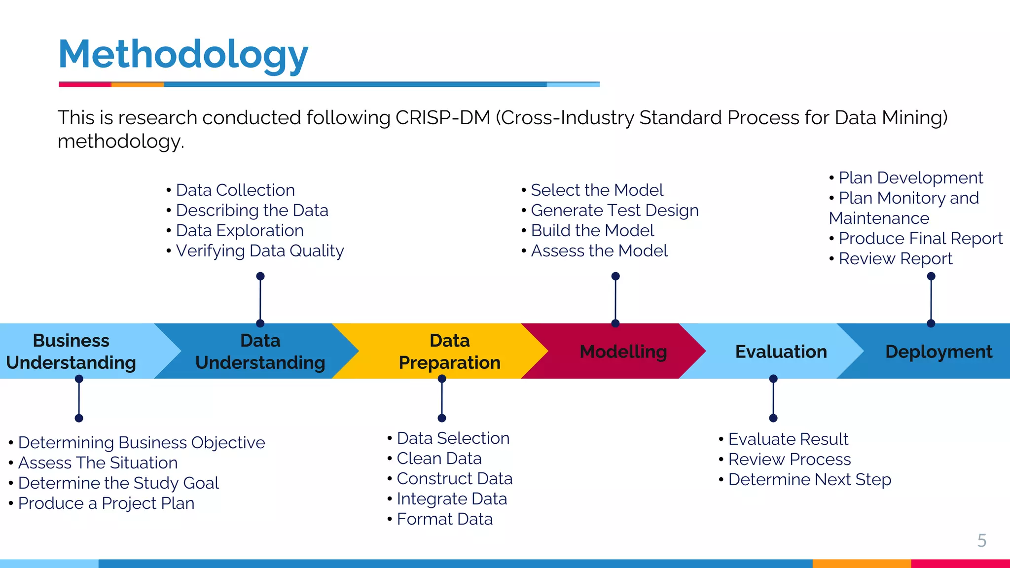
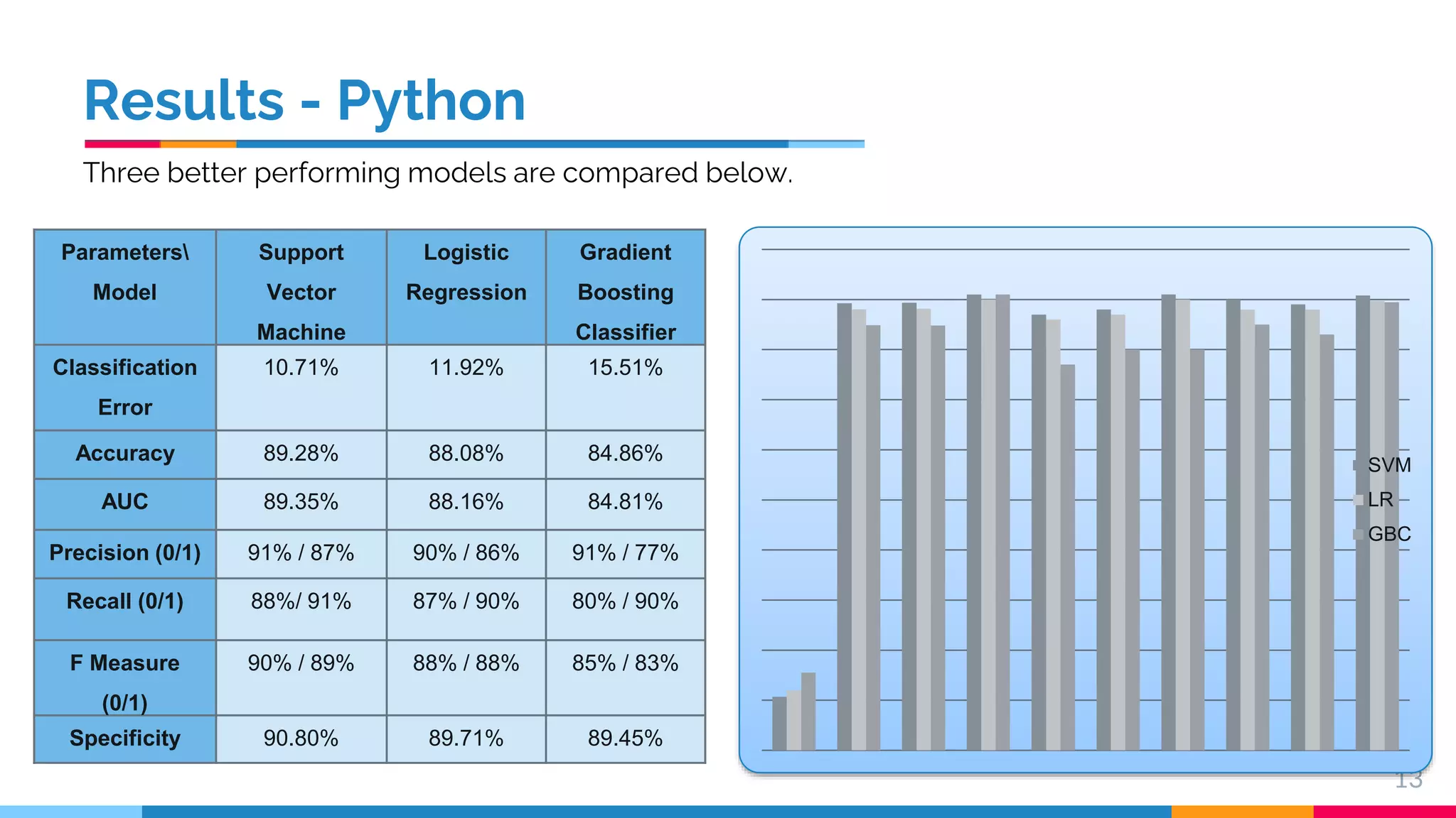
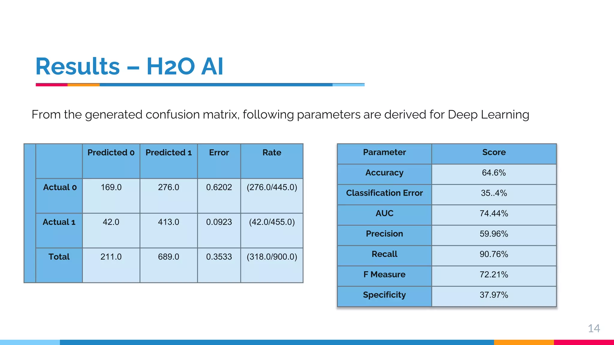
“ Comparative Study of Machine Learning Algorithms for Sentiment Analysis with TF-IDF Vector Creation Sagar Vijay Deogirkar (10547321) MSc Data Analytics Ms. Terri Hoare Supervisor
Index • Introduction • Research Question and Objective • Methodology • Business and Data Understanding • Data Preparation • Modelling • Evaluation • Results • Conclusion and Future Work 2
Introduction Customers are expressing their thoughts about product and offered services more openly than never before. Considering this sentiment analysis is becoming an essential aspect to understand their sentiments. Sentiment analysis cites the use of Natural Language Processing technique to classify the type of sentiment. In other words, Sentiment Analysis is the process to determine if the given text is positive, negative or of neutral sentiment. It is often perform on textual data to help business entities, to monitor their brand’s product or services’ sentiments from client’s reviews. This helps to understand the customer’s requirement which may lead to necessary improvement in product or services if required. 3
Research Question Sentiment Analysis is trending, many programming and non programming platforms have arrived providing solution to this problem. But problem lies with platform selection and more over that, to the model or algorithm selection. The main obstacle is to know, which algorithm can be chosen with TF-IDF vector creation technique, which will lead to determine the class of the sentiment more correctly. 4 Objective The main objective of this research is to compare the State-of-the-Art Deep Learning with Machine Learning algorithms performance on TF-IDF vector creation for Sentiment Analysis.
Methodology Data Understanding 5 Data Preparation Modelling Evaluation Business Understanding Deployment • Determining Business Objective • Assess The Situation • Determine the Study Goal • Produce a Project Plan • Data Selection • Clean Data • Construct Data • Integrate Data • Format Data • Evaluate Result • Review Process • Determine Next Step • Data Collection • Describing the Data • Data Exploration • Verifying Data Quality • Select the Model • Generate Test Design • Build the Model • Assess the Model • Plan Development • Plan Monitory and Maintenance • Produce Final Report • Review Report This is research conducted following CRISP-DM (Cross-Industry Standard Process for Data Mining) methodology.
Business Understanding Sentiment classification is a term which comprises the method to determine the labelled sentiment from the available classes based on the aligned text data. It helps to identify the emotions i.e. sentiment behind the text of high volume data. Text data could be reviews from YouTube, or from any social media platform, or tweets on trending topic involving different hash tags and etc, or articles or news report or such which is in the form of text. 6 Data Understanding • For this research “Twitter Airline” dataset is used. • Dataset comprises of total 14 features and a label, having a total of 14640 rows. • Column Names - tweet id, airline sentiment, airline sentiment confidence, airline sentiment gold, negative reason, negative reason confidence, airline, name, negative reason gold, re tweet count, text, tweet coord, tweet created, tweet location, user time zone. •Sentiment Distribution: 9178 – Negative, 3099 – Neutral and 2363 - Positive. • From the above features only airline_sentiment and text is selected for the research.
Data Preparation • Text Pre-processing – Lowercasing is done. Unnecessary symbols and numbers are removed. • Sentiment Class Filtering - Neutral class’s sentiment is filtered and positive is turned to 1 and Negative to 0. • Data Balancing – Positive and Negative class sentiment is balanced to same number of samples. • Removing Stop Words – Common words in the language are removed. • Text Stemming – Porter Stemming is used to make word into its original form. • Tokenization – Every word is separated in the document. • TF-IDF vector – TF- IDF word vector is created having all the words in the data set with their weight. 7 Text Cleaning Text Processing Vector Creation Data Importation TF- IDF Vector Creation • Text Stemming • Tokenization • Data Balancing • Lowercasing • Removing Symbols and Numbers • Removing Stop Words. Data Importation to the Platform and Considering the Features and label.
Modelling • Selected Models are: Naive Bayes, Support Vector Machine (SVM), Generalised Linear Model (GLM), Logistic Regression, Decision Tree, Random Forest, Gradient Boosted Trees, and Deep Learning. • On Rapid Miner Auto Model is used with 3000 samples. •Deep learning (Neural Network) is observed on H2O AI platform with 3000 samples processed and saved from Rapid Miner. • On Python 4726 samples are used for modelling on above mentioned models. 8
Evaluation Performance of the model is evaluated by generating/calculating following parameters: • Classification Error – It is the total number of error made by the machine learning model to predict correct data from the total number of predicted samples. • Accuracy - Accuracy is the fraction of correct prediction made by the model to the total number of the samples. • AUC - It is the complete area under the 2-dimensional area under the ROC (Receiver Operating Characteristic) curve. • Precision - Precision is the measure of a model which represents the actual positive values predicted by the model from the total positive values. • Recall/Sensitivity - It is the measure of a model which represents the total number of actual positive values predicted by the model. • F1 Score - It is the harmonic mean between precision and recall. • Specificity - It is defined as the ration of the true negative prediction made by the model to the total number of negative values available in the set. 9
Results – Rapid Miner 10 Parameter/ Model NV GLM LR FLM DT RF GBT SVM DL Classification Error 49.6% (+/-) 0.7% 28.7% (+/-) 0.7% 28.7% (+/-) 0.7% 28.7% (+/-) 0.8% 29.2% (+/-) 0.9% 29.9% (+/-) 0.7% 24.5% (+/-) 1.1% 30.6% (+/-) 0.4% 25.9% (+/-) 1.8% Accuracy 50.3% (+/-) 0.7% 71.2% (+/-) 0.7% 71.2% (+/-) 0.7% 72% (+/-) 0.8% 70.7% (+/-) 0.9% 70% (+/-) 0.7% 75.4% (+/-) 1.1% 69.3% (+/-) 0.4% 74.1% (+/-) 1.8% AUC 7.6% (+/-) 2.3% 81.3% (+/-) 2.8% 81.3% (+/-) 2.8% 81.3% (+/-) 2.6% 71.07% (+/-) 1.6% 78.7% (+/-) 2.5% 81.6% (+/-) 1.1% 79.3% (+/-) 2.3% 82.2% (+/-) 2.5% Precision 49.6% (+/-) 0.8% 88.2% (+/-) 2.4% 88.2% (+/-) 2.4% 85.5% (+/-) 4.7% 87.3% (+/-) 4.2% 84% (+/-) 3.8% 77.4% (+/-) 2.6% 65.7% (+/-) 2.3% 83.4% (+/-) 5.8% Recall (Sensitivity) 99.5% (+/-) 0.6% 47.5% (+/-) 3.2% 47.5% (+/-) 3.2% 50.6% (+/-) 2.9% 45.8% (+/-) 3.7% 46.6% (+/-) 3.6% 72.7% (+/-) 4.3% 77.5% (+/-) 5.7% 58.2% (+/-) 3.1% F Measure 66.2% (+/-) 0.7% 61.7% (+/-) 2.4% 61.7% (+/-) 2.4% 63.4% (+/-) 2% 60% (+/-) 2.8% 59.8% (+/-) 2.5% 74.9% (+/-) 2.5% 71% (+/-) 1.6% 68.4% (+/-) 1.8% Specificity 3.1% (+/-) 3% 93.8% (+/-) 1.6% 93.8% (+/-) 1.6% 91.% (+/-) 3% 93.7% (+/-) 2.5% 91.7% (+/-) 2.5% 78% (+/-) 3.4% 61.7% (+/-) 4.7% 89.0% (+/-) 4.3% Result observed on Rapid Miner’s Auto Model are given below.
Results – Rapid Miner 11 Parameters Model Gradient Boosting Trees Deep Learning Classification Error 24.53% (+/-) 1.1% 25.9% (+/-) 1.8% Accuracy 75.46% (+/-) 1.1% 74.1% (+/-) 1.8% AUC 81.6% (+/-) 1.1% 82.2% (+/-) 2.5% Precision 77.4% (+/-) 2.6% 83.4% (+/-) 5.8% Recall (Sensitivity) 72.7% (+/-) 4.3% 58.2% (+/-) 3.1% F Measure 74.9% (+/-) 2.5% 68.4% (+/-) 1.8% Specificity 78% (+/-) 3.4% 89.0% (+/-) 4.3% GBT DL Two better performing models are compared below.
Results - Python 12 Parameters Model SVM GBC (M)NB DT RF LR Classification Error 10.71% 15.51% 13.04% 17.98% 13.32% 11.92% Accuracy 89.28% 84.86% 86.95% 82.72% 86.11% 88.08% AUC 89.35% 84.81% 87.03% 81.72% 85.69% 88.16% Precision (0/1) 91% / 87% 91% / 77% 89% / 85% 81% / 84% 87% / 85% 90% / 86% Recall (0/1) (Sensitivity) 88%/ 91% 80% / 90% 86% / 89% 84% / 82% 85% / 87% 87% / 90% F Measure (0/1) 90% / 89% 85% / 83% 87% / 87% 83% / 83% 86% / 86% 88% / 88% Specificity 90.80% 89.45% 88.52% 81.12% 86.38% 89.71% Result observed on Python are given below.
Results - Python 13 Parameters Model Support Vector Machine Logistic Regression Gradient Boosting Classifier Classification Error 10.71% 11.92% 15.51% Accuracy 89.28% 88.08% 84.86% AUC 89.35% 88.16% 84.81% Precision (0/1) 91% / 87% 90% / 86% 91% / 77% Recall (0/1) 88%/ 91% 87% / 90% 80% / 90% F Measure (0/1) 90% / 89% 88% / 88% 85% / 83% Specificity 90.80% 89.71% 89.45% SVM LR GBC Three better performing models are compared below.
Results – H2O AI 14 Predicted 0 Predicted 1 Error Rate Actual 0 169.0 276.0 0.6202 (276.0/445.0) Actual 1 42.0 413.0 0.0923 (42.0/455.0) Total 211.0 689.0 0.3533 (318.0/900.0) From the generated confusion matrix, following parameters are derived for Deep Learning Parameter Score Accuracy 64.6% Classification Error 35..4% AUC 74.44% Precision 59.96% Recall 90.76% F Measure 72.21% Specificity 37.97%
Results – Overall 15 •On Rapid Miner there is not so much difference in Classification Error, Accuracy, and AUC between Gradient Boosting Tree (GBT) and Deep Learning (DL) models, which are one of the most important evaluation criteria in machine learning classification algorithms. • Support Vector Machine is clearly outperforming every other traditional machine learning classification model on Python. • Either of the better performing model on Rapid Miner has not performed well with more number of samples on python platform or on H2O AI. • Support Vector Machine has got more score in all classification evaluating parameters. • Deep Learning model on H20 AI is giving unfavourable results if compared with the considered hypothesis. • The results from Deep Learning model on H20 platform do not outperform the Rapid Miner’s Auto model results.
Conclusion and Future Work 16 • From above results and discussion we can observe that Support Vector Machine model is performing better than other State-of-the-Art models with TF-IDF word vector creation. • Rapid Miner auto model’s score can be used as a bench mark for all the platforms and model. Different results can be observed depending on the number of samples. • The future work for this study will involve the use of Recurrent Neural Network with Keras for sentiment classification. • It also involves the use of different word vector creating technique such as Term Frequency (TF), Term Occurrence (TO), and Binary Term Occurrence (BTO).
Thank You

Comparative Study of Machine Learning Algorithms for Sentiment Analysis with TF-IDF Vector Creation

  • 1.
    “ Comparative Study ofMachine Learning Algorithms for Sentiment Analysis with TF-IDF Vector Creation Sagar Vijay Deogirkar (10547321) MSc Data Analytics Ms. Terri Hoare Supervisor
  • 2.
    Index • Introduction • ResearchQuestion and Objective • Methodology • Business and Data Understanding • Data Preparation • Modelling • Evaluation • Results • Conclusion and Future Work 2
  • 3.
    Introduction Customers are expressingtheir thoughts about product and offered services more openly than never before. Considering this sentiment analysis is becoming an essential aspect to understand their sentiments. Sentiment analysis cites the use of Natural Language Processing technique to classify the type of sentiment. In other words, Sentiment Analysis is the process to determine if the given text is positive, negative or of neutral sentiment. It is often perform on textual data to help business entities, to monitor their brand’s product or services’ sentiments from client’s reviews. This helps to understand the customer’s requirement which may lead to necessary improvement in product or services if required. 3
  • 4.
    Research Question Sentiment Analysisis trending, many programming and non programming platforms have arrived providing solution to this problem. But problem lies with platform selection and more over that, to the model or algorithm selection. The main obstacle is to know, which algorithm can be chosen with TF-IDF vector creation technique, which will lead to determine the class of the sentiment more correctly. 4 Objective The main objective of this research is to compare the State-of-the-Art Deep Learning with Machine Learning algorithms performance on TF-IDF vector creation for Sentiment Analysis.
  • 5.
    Methodology Data Understanding 5 Data Preparation Modelling Evaluation Business Understanding Deployment • DeterminingBusiness Objective • Assess The Situation • Determine the Study Goal • Produce a Project Plan • Data Selection • Clean Data • Construct Data • Integrate Data • Format Data • Evaluate Result • Review Process • Determine Next Step • Data Collection • Describing the Data • Data Exploration • Verifying Data Quality • Select the Model • Generate Test Design • Build the Model • Assess the Model • Plan Development • Plan Monitory and Maintenance • Produce Final Report • Review Report This is research conducted following CRISP-DM (Cross-Industry Standard Process for Data Mining) methodology.
  • 6.
    Business Understanding Sentiment classificationis a term which comprises the method to determine the labelled sentiment from the available classes based on the aligned text data. It helps to identify the emotions i.e. sentiment behind the text of high volume data. Text data could be reviews from YouTube, or from any social media platform, or tweets on trending topic involving different hash tags and etc, or articles or news report or such which is in the form of text. 6 Data Understanding • For this research “Twitter Airline” dataset is used. • Dataset comprises of total 14 features and a label, having a total of 14640 rows. • Column Names - tweet id, airline sentiment, airline sentiment confidence, airline sentiment gold, negative reason, negative reason confidence, airline, name, negative reason gold, re tweet count, text, tweet coord, tweet created, tweet location, user time zone. •Sentiment Distribution: 9178 – Negative, 3099 – Neutral and 2363 - Positive. • From the above features only airline_sentiment and text is selected for the research.
  • 7.
    Data Preparation • TextPre-processing – Lowercasing is done. Unnecessary symbols and numbers are removed. • Sentiment Class Filtering - Neutral class’s sentiment is filtered and positive is turned to 1 and Negative to 0. • Data Balancing – Positive and Negative class sentiment is balanced to same number of samples. • Removing Stop Words – Common words in the language are removed. • Text Stemming – Porter Stemming is used to make word into its original form. • Tokenization – Every word is separated in the document. • TF-IDF vector – TF- IDF word vector is created having all the words in the data set with their weight. 7 Text Cleaning Text Processing Vector Creation Data Importation TF- IDF Vector Creation • Text Stemming • Tokenization • Data Balancing • Lowercasing • Removing Symbols and Numbers • Removing Stop Words. Data Importation to the Platform and Considering the Features and label.
  • 8.
    Modelling • Selected Modelsare: Naive Bayes, Support Vector Machine (SVM), Generalised Linear Model (GLM), Logistic Regression, Decision Tree, Random Forest, Gradient Boosted Trees, and Deep Learning. • On Rapid Miner Auto Model is used with 3000 samples. •Deep learning (Neural Network) is observed on H2O AI platform with 3000 samples processed and saved from Rapid Miner. • On Python 4726 samples are used for modelling on above mentioned models. 8
  • 9.
    Evaluation Performance of themodel is evaluated by generating/calculating following parameters: • Classification Error – It is the total number of error made by the machine learning model to predict correct data from the total number of predicted samples. • Accuracy - Accuracy is the fraction of correct prediction made by the model to the total number of the samples. • AUC - It is the complete area under the 2-dimensional area under the ROC (Receiver Operating Characteristic) curve. • Precision - Precision is the measure of a model which represents the actual positive values predicted by the model from the total positive values. • Recall/Sensitivity - It is the measure of a model which represents the total number of actual positive values predicted by the model. • F1 Score - It is the harmonic mean between precision and recall. • Specificity - It is defined as the ration of the true negative prediction made by the model to the total number of negative values available in the set. 9
  • 10.
    Results – RapidMiner 10 Parameter/ Model NV GLM LR FLM DT RF GBT SVM DL Classification Error 49.6% (+/-) 0.7% 28.7% (+/-) 0.7% 28.7% (+/-) 0.7% 28.7% (+/-) 0.8% 29.2% (+/-) 0.9% 29.9% (+/-) 0.7% 24.5% (+/-) 1.1% 30.6% (+/-) 0.4% 25.9% (+/-) 1.8% Accuracy 50.3% (+/-) 0.7% 71.2% (+/-) 0.7% 71.2% (+/-) 0.7% 72% (+/-) 0.8% 70.7% (+/-) 0.9% 70% (+/-) 0.7% 75.4% (+/-) 1.1% 69.3% (+/-) 0.4% 74.1% (+/-) 1.8% AUC 7.6% (+/-) 2.3% 81.3% (+/-) 2.8% 81.3% (+/-) 2.8% 81.3% (+/-) 2.6% 71.07% (+/-) 1.6% 78.7% (+/-) 2.5% 81.6% (+/-) 1.1% 79.3% (+/-) 2.3% 82.2% (+/-) 2.5% Precision 49.6% (+/-) 0.8% 88.2% (+/-) 2.4% 88.2% (+/-) 2.4% 85.5% (+/-) 4.7% 87.3% (+/-) 4.2% 84% (+/-) 3.8% 77.4% (+/-) 2.6% 65.7% (+/-) 2.3% 83.4% (+/-) 5.8% Recall (Sensitivity) 99.5% (+/-) 0.6% 47.5% (+/-) 3.2% 47.5% (+/-) 3.2% 50.6% (+/-) 2.9% 45.8% (+/-) 3.7% 46.6% (+/-) 3.6% 72.7% (+/-) 4.3% 77.5% (+/-) 5.7% 58.2% (+/-) 3.1% F Measure 66.2% (+/-) 0.7% 61.7% (+/-) 2.4% 61.7% (+/-) 2.4% 63.4% (+/-) 2% 60% (+/-) 2.8% 59.8% (+/-) 2.5% 74.9% (+/-) 2.5% 71% (+/-) 1.6% 68.4% (+/-) 1.8% Specificity 3.1% (+/-) 3% 93.8% (+/-) 1.6% 93.8% (+/-) 1.6% 91.% (+/-) 3% 93.7% (+/-) 2.5% 91.7% (+/-) 2.5% 78% (+/-) 3.4% 61.7% (+/-) 4.7% 89.0% (+/-) 4.3% Result observed on Rapid Miner’s Auto Model are given below.
  • 11.
    Results – RapidMiner 11 Parameters Model Gradient Boosting Trees Deep Learning Classification Error 24.53% (+/-) 1.1% 25.9% (+/-) 1.8% Accuracy 75.46% (+/-) 1.1% 74.1% (+/-) 1.8% AUC 81.6% (+/-) 1.1% 82.2% (+/-) 2.5% Precision 77.4% (+/-) 2.6% 83.4% (+/-) 5.8% Recall (Sensitivity) 72.7% (+/-) 4.3% 58.2% (+/-) 3.1% F Measure 74.9% (+/-) 2.5% 68.4% (+/-) 1.8% Specificity 78% (+/-) 3.4% 89.0% (+/-) 4.3% GBT DL Two better performing models are compared below.
  • 12.
    Results - Python 12 Parameters Model SVMGBC (M)NB DT RF LR Classification Error 10.71% 15.51% 13.04% 17.98% 13.32% 11.92% Accuracy 89.28% 84.86% 86.95% 82.72% 86.11% 88.08% AUC 89.35% 84.81% 87.03% 81.72% 85.69% 88.16% Precision (0/1) 91% / 87% 91% / 77% 89% / 85% 81% / 84% 87% / 85% 90% / 86% Recall (0/1) (Sensitivity) 88%/ 91% 80% / 90% 86% / 89% 84% / 82% 85% / 87% 87% / 90% F Measure (0/1) 90% / 89% 85% / 83% 87% / 87% 83% / 83% 86% / 86% 88% / 88% Specificity 90.80% 89.45% 88.52% 81.12% 86.38% 89.71% Result observed on Python are given below.
  • 13.
    Results - Python 13 Parameters Model Support Vector Machine Logistic Regression Gradient Boosting Classifier Classification Error 10.71%11.92% 15.51% Accuracy 89.28% 88.08% 84.86% AUC 89.35% 88.16% 84.81% Precision (0/1) 91% / 87% 90% / 86% 91% / 77% Recall (0/1) 88%/ 91% 87% / 90% 80% / 90% F Measure (0/1) 90% / 89% 88% / 88% 85% / 83% Specificity 90.80% 89.71% 89.45% SVM LR GBC Three better performing models are compared below.
  • 14.
    Results – H2OAI 14 Predicted 0 Predicted 1 Error Rate Actual 0 169.0 276.0 0.6202 (276.0/445.0) Actual 1 42.0 413.0 0.0923 (42.0/455.0) Total 211.0 689.0 0.3533 (318.0/900.0) From the generated confusion matrix, following parameters are derived for Deep Learning Parameter Score Accuracy 64.6% Classification Error 35..4% AUC 74.44% Precision 59.96% Recall 90.76% F Measure 72.21% Specificity 37.97%
  • 15.
    Results – Overall 15 •OnRapid Miner there is not so much difference in Classification Error, Accuracy, and AUC between Gradient Boosting Tree (GBT) and Deep Learning (DL) models, which are one of the most important evaluation criteria in machine learning classification algorithms. • Support Vector Machine is clearly outperforming every other traditional machine learning classification model on Python. • Either of the better performing model on Rapid Miner has not performed well with more number of samples on python platform or on H2O AI. • Support Vector Machine has got more score in all classification evaluating parameters. • Deep Learning model on H20 AI is giving unfavourable results if compared with the considered hypothesis. • The results from Deep Learning model on H20 platform do not outperform the Rapid Miner’s Auto model results.
  • 16.
    Conclusion and FutureWork 16 • From above results and discussion we can observe that Support Vector Machine model is performing better than other State-of-the-Art models with TF-IDF word vector creation. • Rapid Miner auto model’s score can be used as a bench mark for all the platforms and model. Different results can be observed depending on the number of samples. • The future work for this study will involve the use of Recurrent Neural Network with Keras for sentiment classification. • It also involves the use of different word vector creating technique such as Term Frequency (TF), Term Occurrence (TO), and Binary Term Occurrence (BTO).
  • 17.