Downloaded 238 times


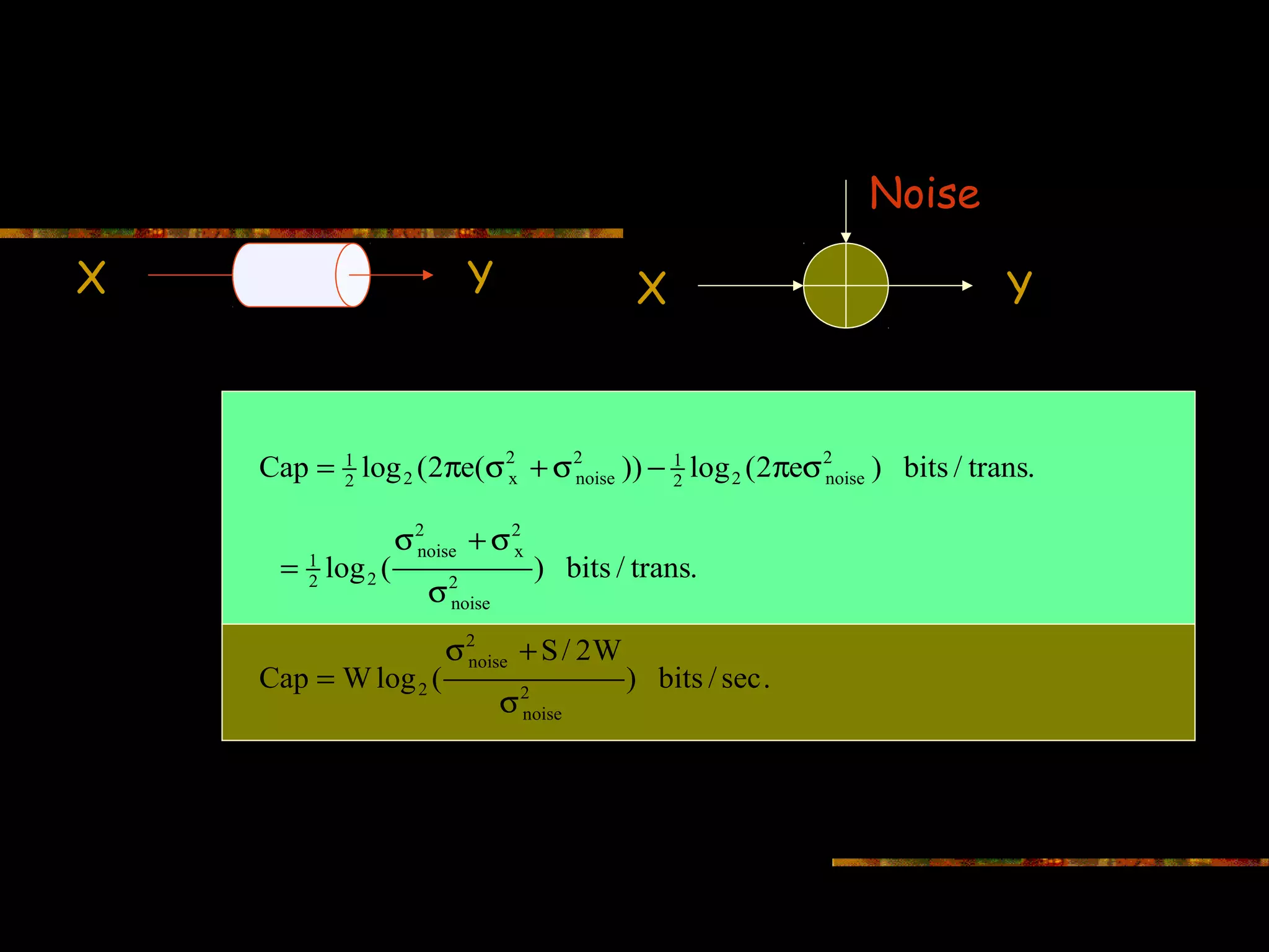
![Capacity for Additive White Gaussian Noise Noise Input X Output Y Cap := sup [H(Y) − H( Noise)] p( x ) x 2 ≤S / 2 W W is (single sided) bandwidth Input X is Gaussian with power spectral density (psd) ≤S/2W; Noise is Gaussian with psd = σ2noise Output Y is Gaussian with psd = σy2 = S/2W + σ2noise For Gaussian Channels: σy2 = σx2 +σnoise2](https://image.slidesharecdn.com/channel-coding-130214001651-phpapp01/75/Channel-coding-29-2048.jpg)


This document introduces information theory and channel capacity models. It discusses several channel models including the binary symmetric channel (BSC), binary erasure channel, and additive white Gaussian noise channel. It explains how channel capacity is defined as the maximum rate of error-free transmission and derives the capacity for some basic channels. The document also covers channel coding techniques like interleaving that can improve performance by converting burst errors into random errors.
Overview of information theory, channel capacity, and models presented by A.J. Han Vinck.
Lecture outline covering models, channel capacity, Shannon's channel coding theorem, and its converse.
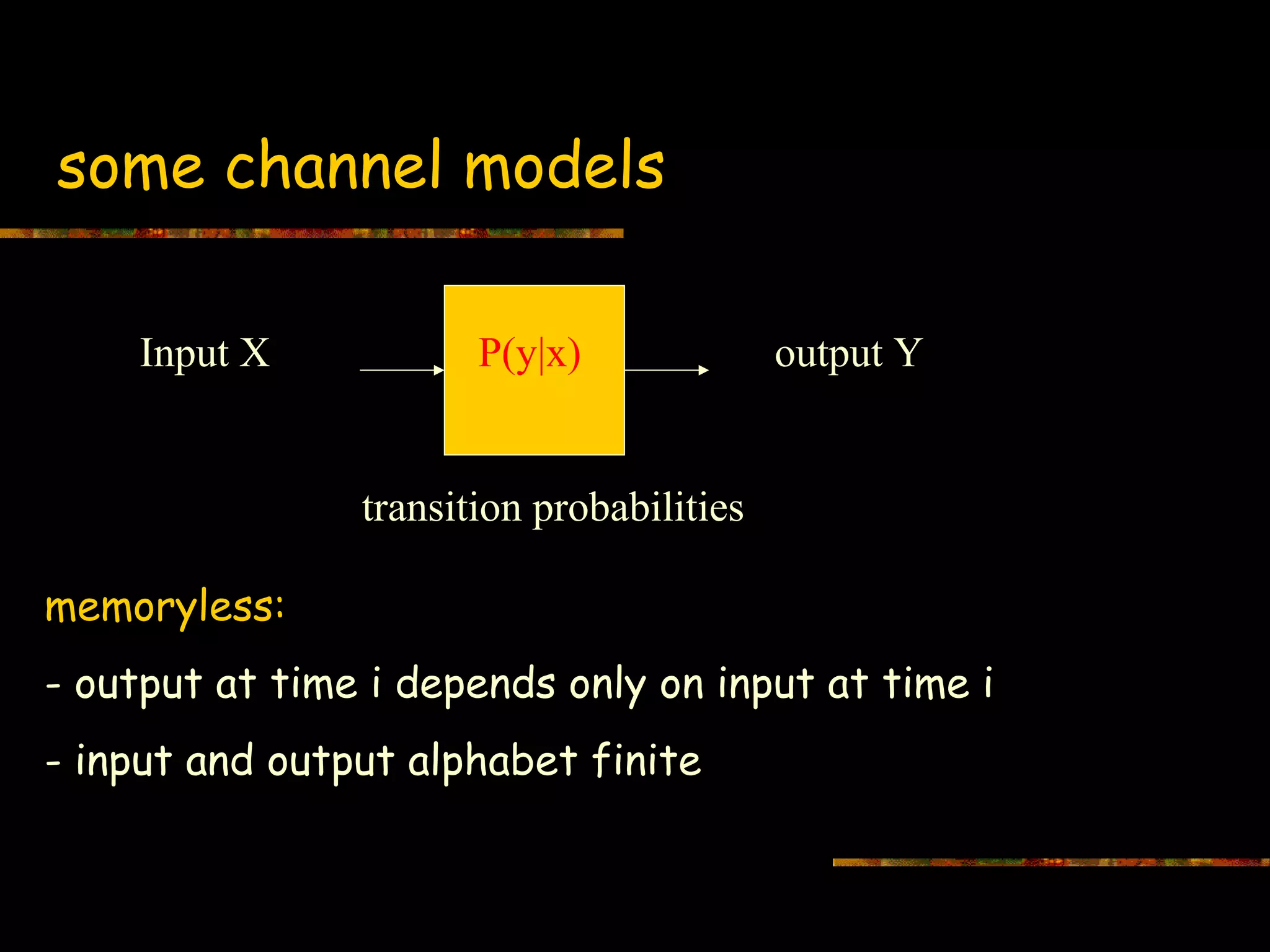
Introduction to channel models including memoryless channels where output depends solely on current input.
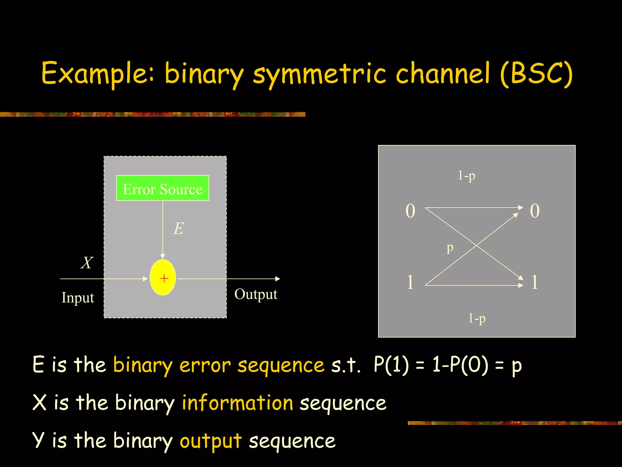
Detailed example of Binary Symmetric Channel (BSC) illustrating error sequences and outputs.
Homework pertains to calculating capacity based on parameters A and σ².
Explores other models like Z-channel and Erasure channel with specified transition probabilities.
Describes the Erasure channel model featuring probabilities with and without errors.
Discusses the Gilbert-Elliot burst error model showing dependency of outputs.
Defines channel capacity with Shannon's equations and emphasizes the role of input probabilities.
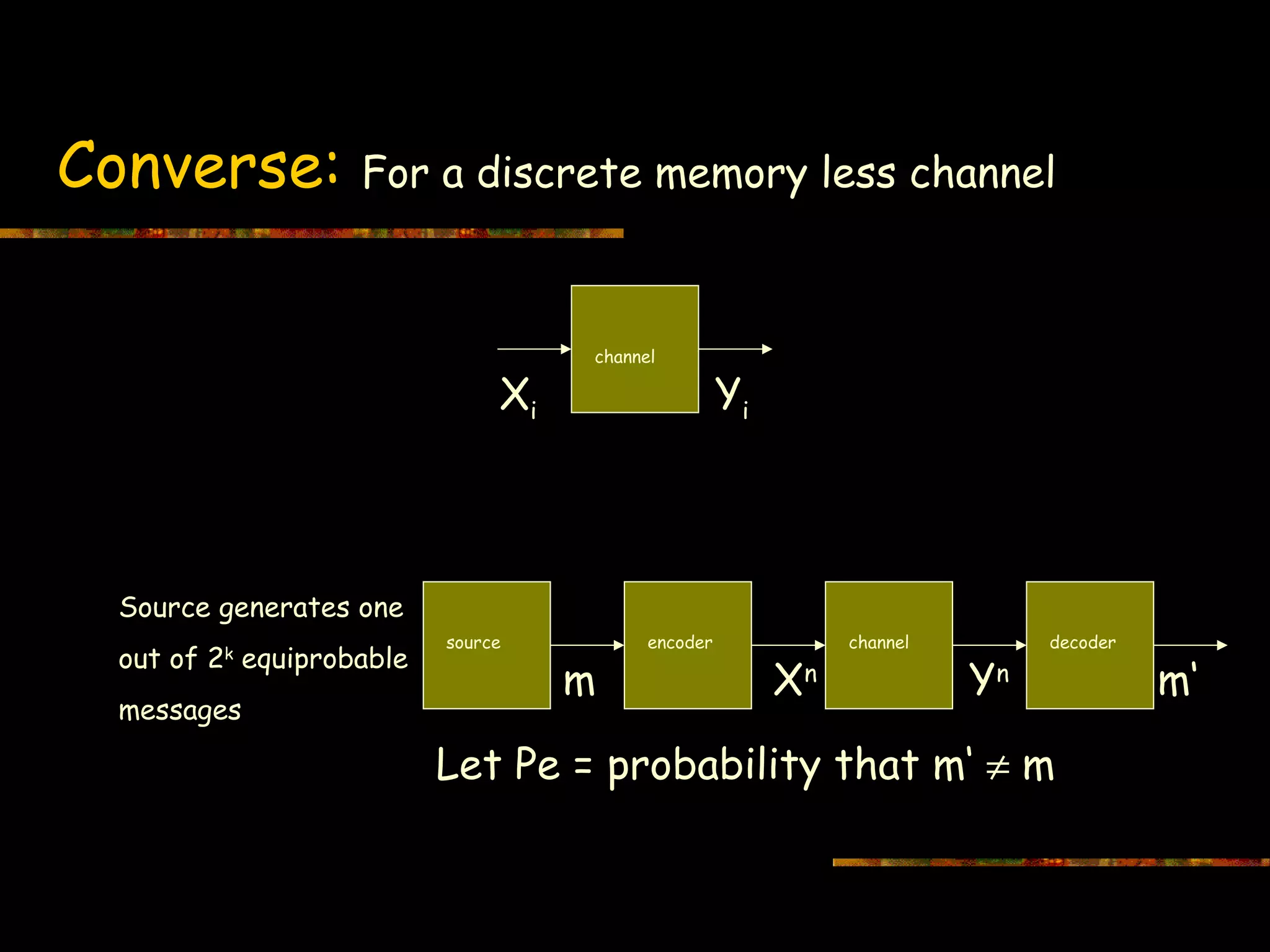
Illustration of code book structure and message transmission with error considerations.
Defines the rate R of a code as the ratio of information bits k to channel uses n, indicating decoding methods.
Details on Shannon's encoding/decoding methods with specific error probabilities.
Mathematical analysis on decoding error probabilities and their limits as n approaches infinity.
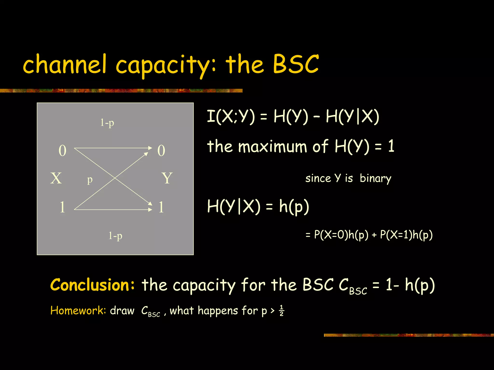
Introduces capacity calculations for BSC and sets up further homework on capacity behavior.
Graphical representation shows the relationship between channel capacity and bit error rate.
Discussion of Z-channel in optical communications with a focus on maximizing channel capacity.
Erasure channel capacity calculations relevant for CDMA detection, emphasizing potential capacity outcomes.
Homework assignment focusing on calculating capacity for the channel model with errors.
Presents an example to maximize H(Y) - H(Y|X) given probabilities and hints on calculus applications.
General diagram representation of channel models including inputs, outputs, and transition probability.
Indicates that I(X;Y) is convex based on input probabilities, simplifying maximization.
Explains error probability conditions for rates exceeding channel capacity.
Mathematical framework detailing relationships between inputs and outputs in a discrete memoryless channel.
Further analysis on error probability in relation to channel capacity, emphasizing outcomes for large n.
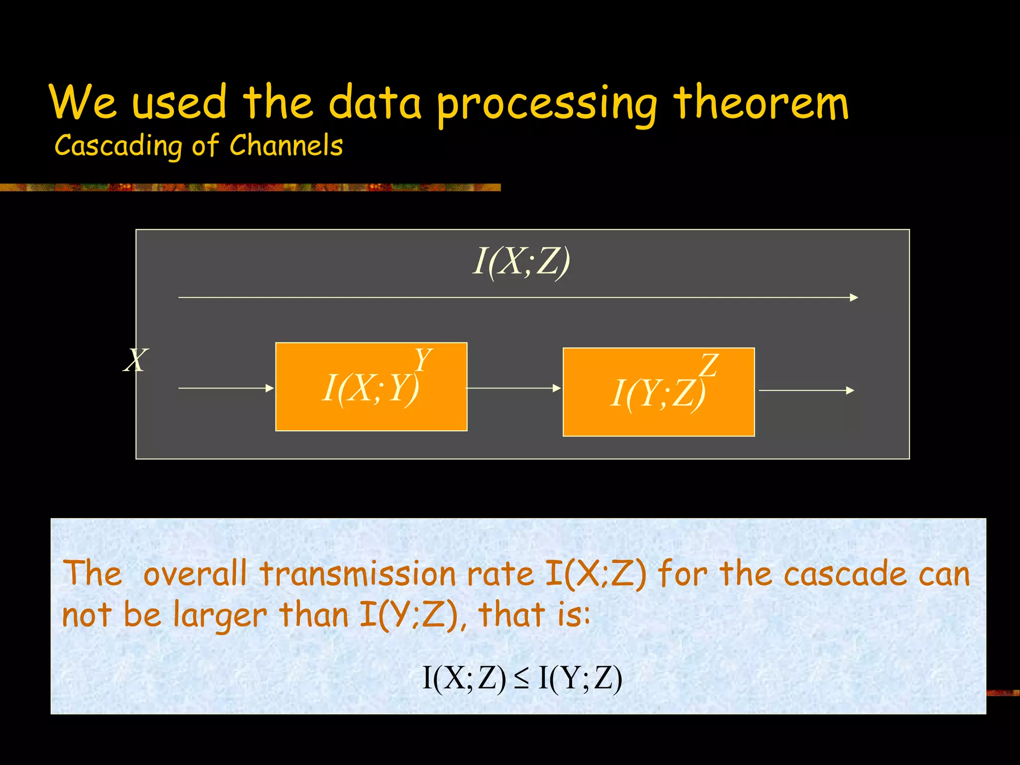
Discusses the impact of cascading channels on overall transmission rates using mutual information.
Introduces underlying probability theories leveraging the weak law of large numbers for large sequences.
Details consequences of probabilistic outcomes over large n, introducing entropy calculations.
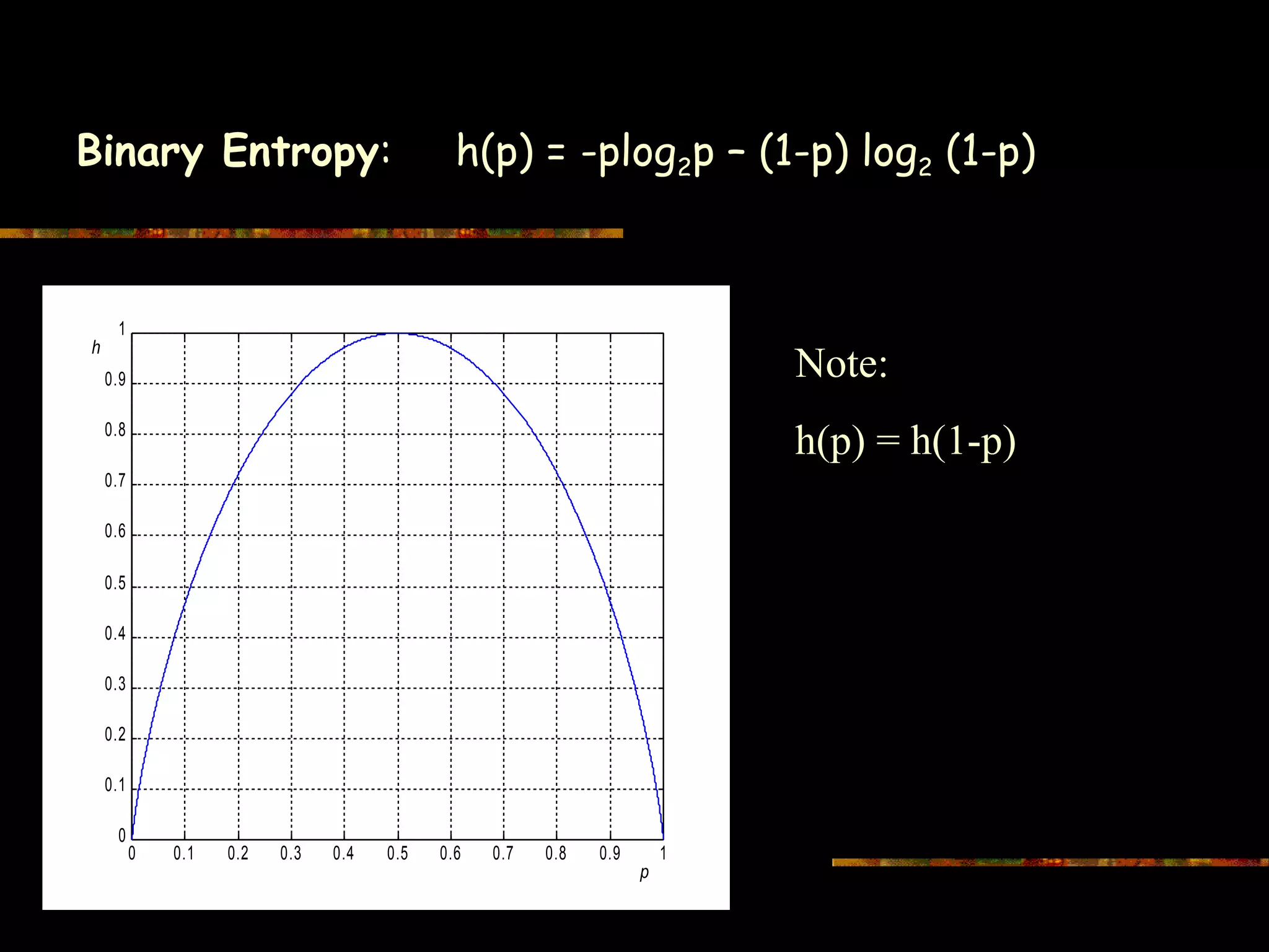
Defines the binary entropy function h(p) and its symmetrical properties with graphical representation.
Defines capacity in the context of AWGN channels including variables of noise and bandwidth.
Specific equations for calculating channel capacity in Gaussian conditions.
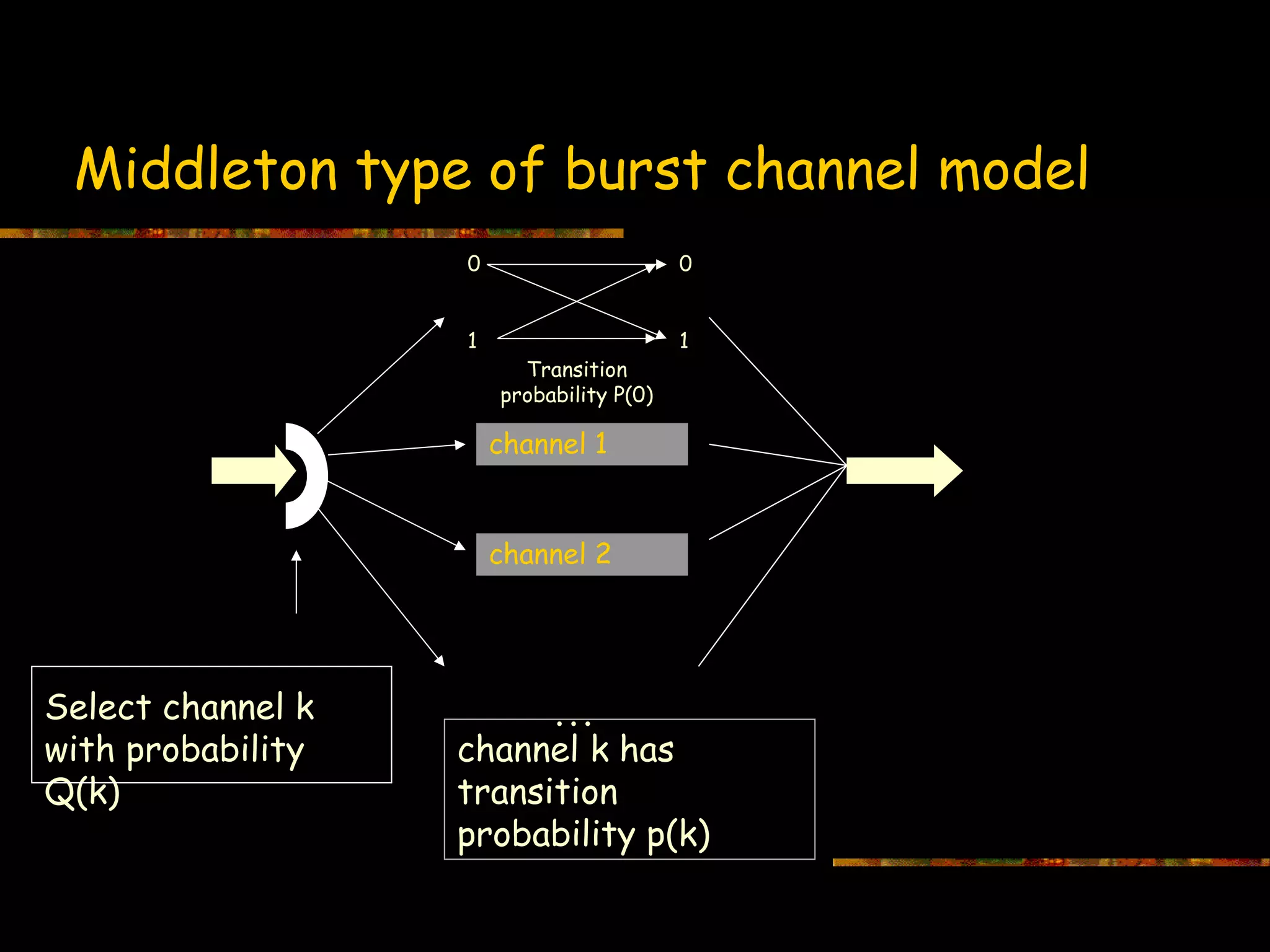
Middleton type burst channel model presenting transition probabilities for selected channels.
Describes the Fritzman model with multiple states closer to real-world scenarios.
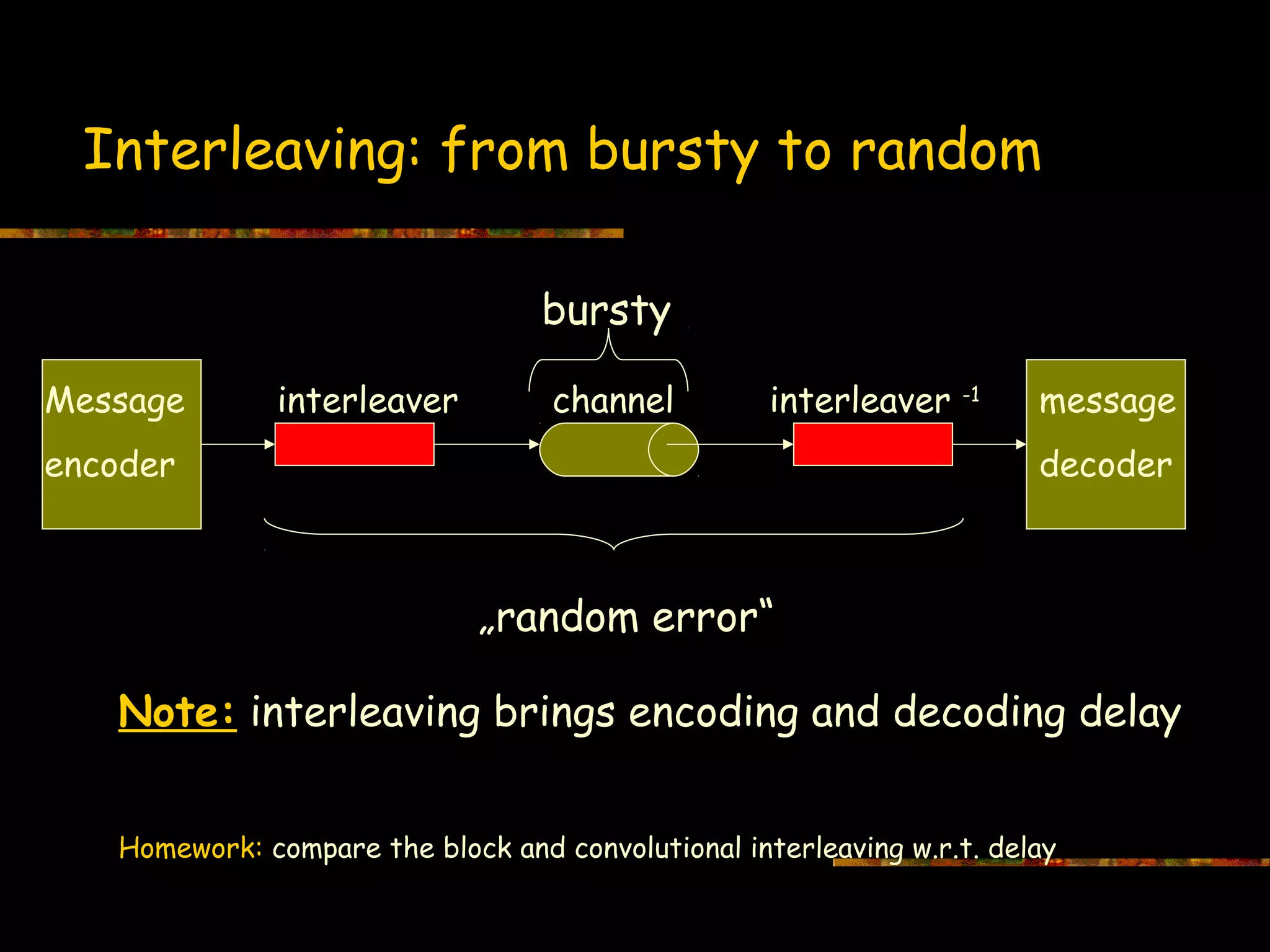
Explains interleaving as a technique to convert burst errors to random errors and associated delays.
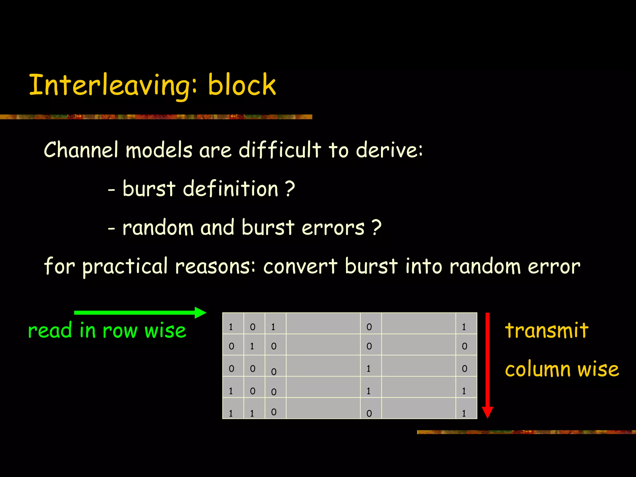
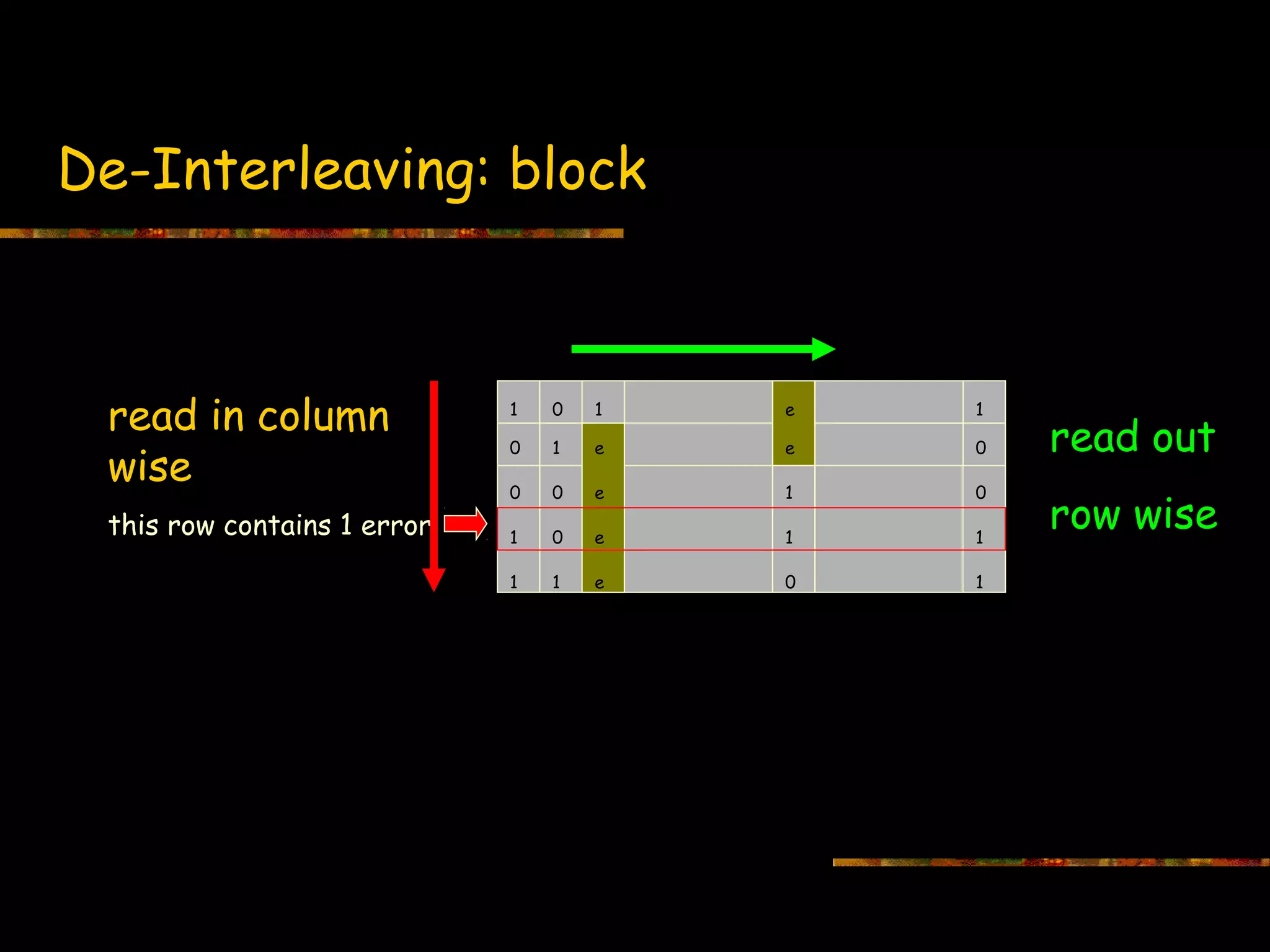
Description of block interleaving techniques to manage bursty errors by changing reading order.
Illustrates the de-interleaving process, detailing how error readings can be organized.
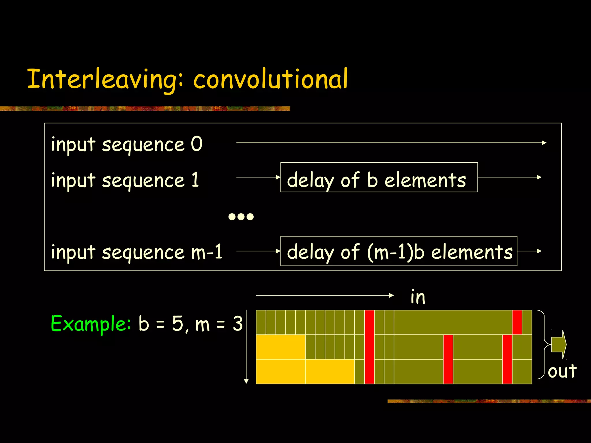
Explains convolutional interleaving with examples highlighting delay in processing.