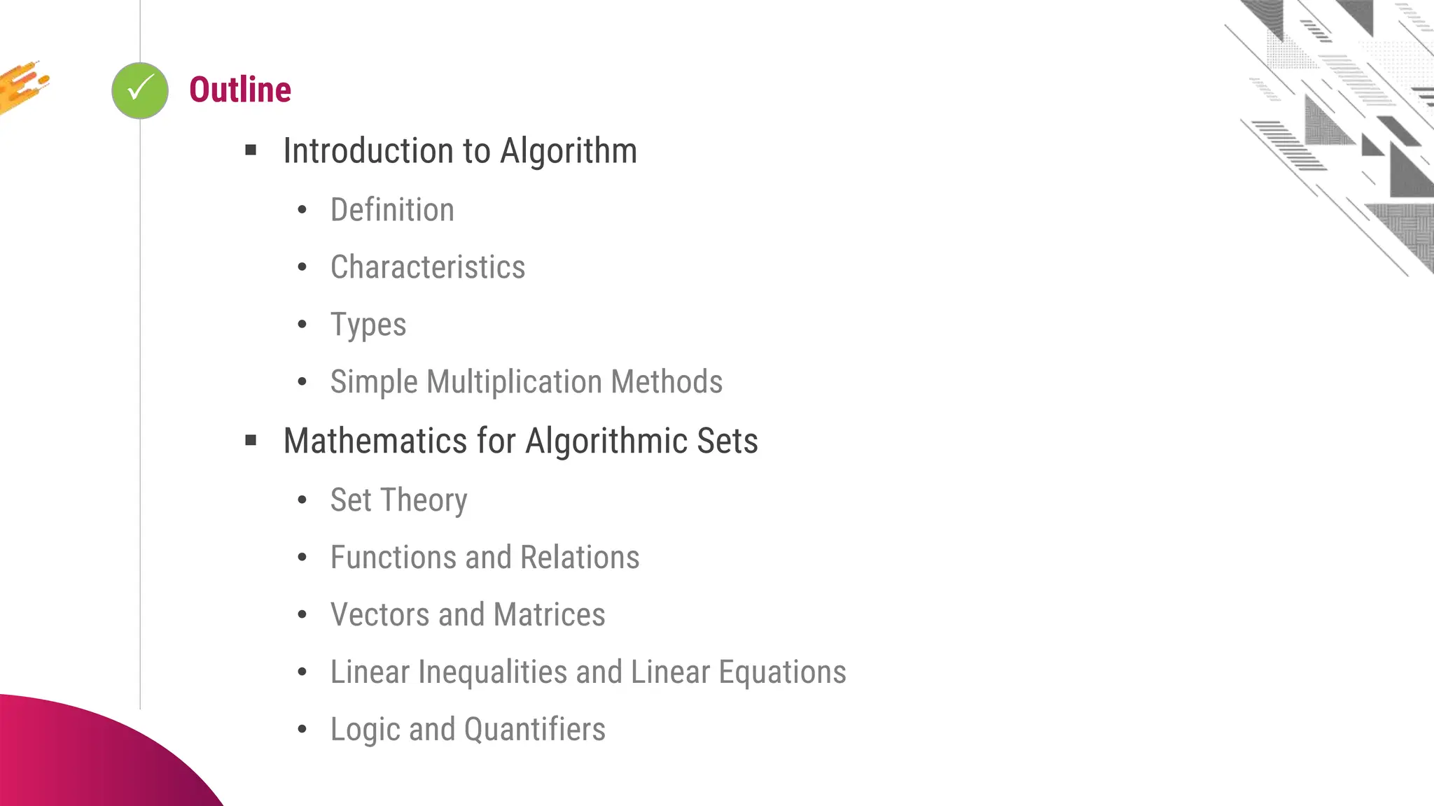
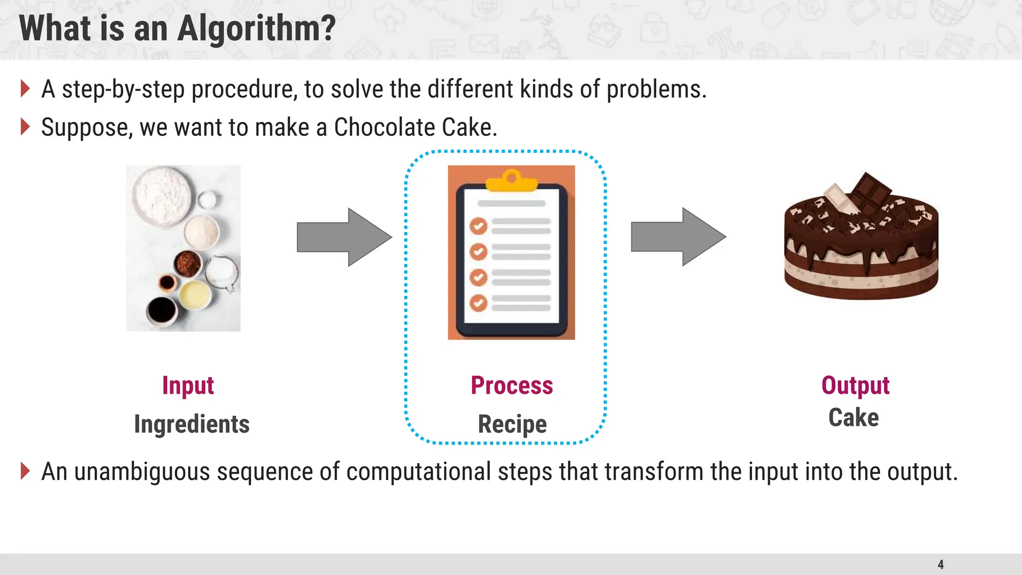
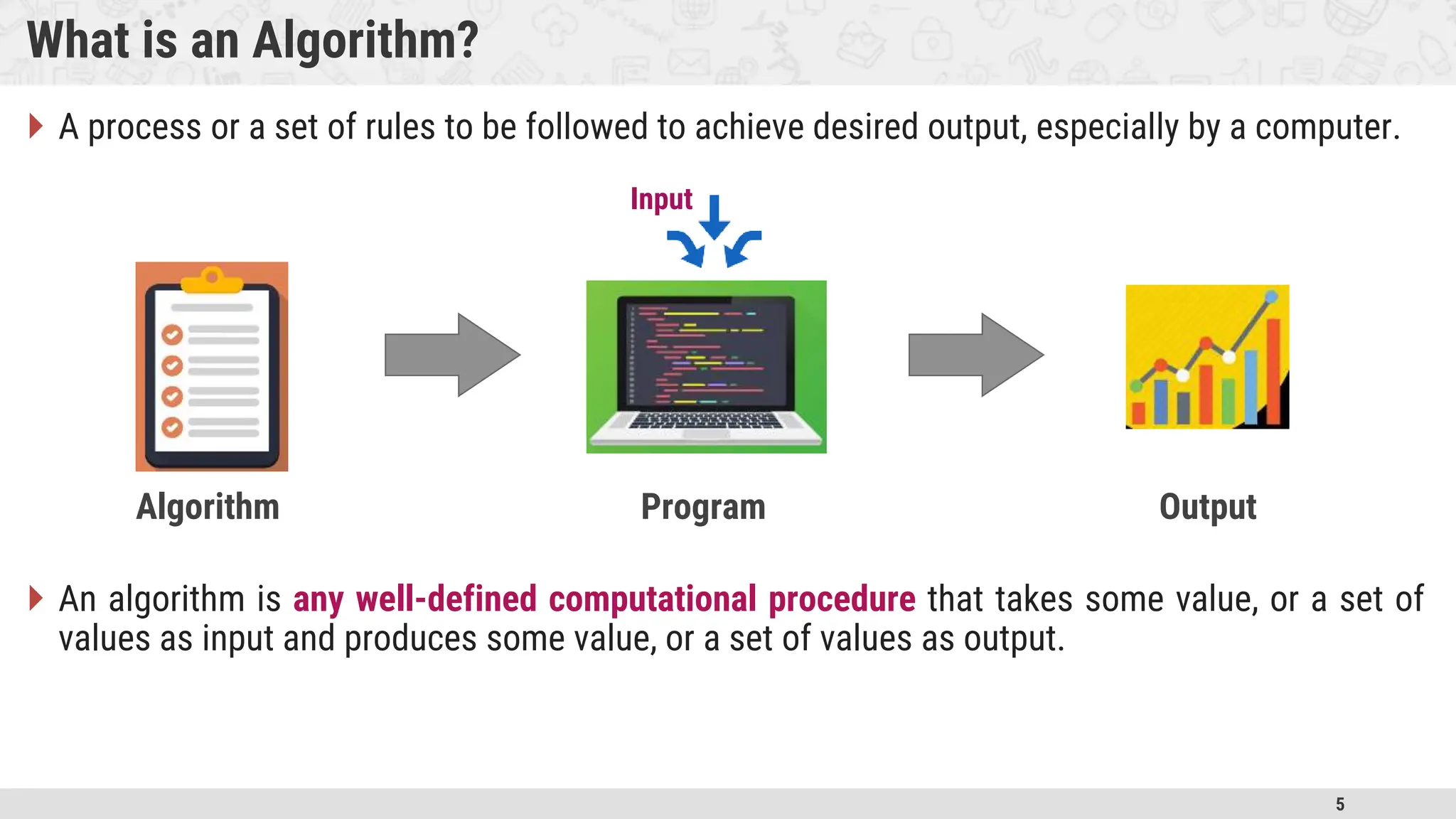
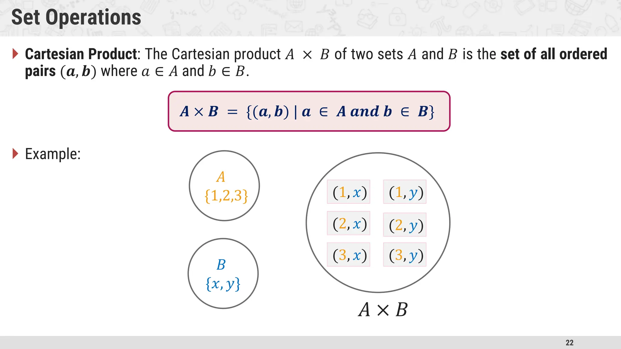
Unit-1: Basics of Algorithms and Mathematics
 Looping Outline  Introduction to Algorithm • Definition • Characteristics • Types • Simple Multiplication Methods  Mathematics for Algorithmic Sets • Set Theory • Functions and Relations • Vectors and Matrices • Linear Inequalities and Linear Equations • Logic and Quantifiers
4 What is an Algorithm?  A step-by-step procedure, to solve the different kinds of problems.  Suppose, we want to make a Chocolate Cake.  An unambiguous sequence of computational steps that transform the input into the output. Output Input Process Ingredients Recipe Cake
5 What is an Algorithm?  A process or a set of rules to be followed to achieve desired output, especially by a computer.  An algorithm is any well-defined computational procedure that takes some value, or a set of values as input and produces some value, or a set of values as output. Output Algorithm Program Input
6 Characteristics of An Algorithm  Finiteness: An algorithm must always terminate after a finite number of steps.  Definiteness: Each step of an algorithm must be precisely defined.  Input: An algorithm has zero or more inputs.  Output: An algorithm must have at least one desirable output.  Effectiveness: All the operations to be performed in the algorithm must be sufficiently basic so that they can, in principle be done exactly and in a finite length of time.
7 Types of Algorithm  Simple recursive algorithms  Backtracking algorithms  Divide and conquer algorithms  Dynamic programming algorithms  Greedy algorithms  Branch and bound algorithms  Brute force algorithms  Randomized algorithms
8 Simple Multiplication Methods 1. American approach 2. English approach 9 8 1 3 9 2 4 2 9 4 3 1 9 6 2 9 8 1 1 2 1 0 5 5 4 4 3 2 1 9 8 1 3 9 2 4 2 9 4 3 1 9 6 2 9 8 1 1 2 1 0 5 5 4 4 3 2 1
9 Simple Multiplication Methods 3. à 𝒍𝒂 𝒓𝒖𝒔𝒔𝒆 multiplication i. Write the multiplicand and multiplier side by side. ii. Make two columns, one under each operand. iii. Repeat step iv and v until the number in the left column is 1. iv. Divide the number in the left hand column by 2, ignoring any fractions. v. Double the number in the right hand column by adding it to itself. vi. Next cross out each row where the number in the left hand column is even. vii. Finally add up the numbers that remain in the right hand column. 1234 2468 4936 9872 19744 39488 78976 157952 315904 631808 981 490 245 122 61 30 15 7 3 1 1234 4936 19744 78976 157952 315904 631808 1210554
10 Simple Multiplication Methods 4. Multiplication by divide and conquer  Both the multiplicand and the multiplier must have the same number of digits and this number be a power of 2. If not then it can be done by adding zeros on the left if necessary. Multiply Shift Result (09) * (12) 4 (09) * (34) 2 (81) * (12) 2 (81) * (34) 0 . . . . 8 0 1 . . 6 0 3 . . 2 7 9 5 4 7 2 1 2 1 0 5 5 4 Multiplier 1 2 3 4 Multiplicand 0 9 8 1 i. Multiply left half of the multiplicand by left half of multiplier and shift the result by no. of digits of multiplier i.e. 4. ii. Multiply left half of the multiplicand by right half of the multiplier, shift the result by half the number of digits of multiplier i.e. 2. iii. Multiply right half of the multiplicand by left half of the multiplier, shift the result by half the number of digits of multiplier i.e. 2. iv. Multiply right half of the multiplicand by right half of the multiplier the result is not shifted at all.
12 Set Theory  A set is an unordered collection of distinct objects.  The objects in a set are called elements or members of the set. Example 1 Set A = 11, 12, 21, 22 Set B = 5, 10, 15, 20, 25 Set C = x x is an odd integer greater than 1} Set D = {x | x ∈ C and x ≤ 11} Example 2 Roster Notation Set-builder Notation
13 Set Theory  Finite & Infinite sets: A set is finite if it contains a finite number of elements, otherwise it is an infinite set.  Subset: For two sets 𝐴 and 𝐶, we say that 𝐶 is a subset of 𝐴, written as 𝐶⊆𝐴, if each member of set 𝐶 is also a member of set 𝐴. Example 1 A = 𝑥 𝑥 ∈ Z and 𝑥2 − 81 = 0} A = −9,9 B = 𝑥 𝑥 is divisible by 2} B = {2,4,6, … , } Example 2 Set 𝐀 is a finite set Set 𝐁 is an infinite set
14 Set Theory  Proper Subset: A proper subset of a set 𝐴 is a subset of 𝐴 that is not equal to 𝐴. Example 1 If 𝐴 = {1,3,5} and 𝐵 = 1,5 Then set 𝐵 is a proper subset of 𝐴. If 𝐴 = {1,3,5} and 𝐶 = 1,3,5 Then set C is a subset of 𝐴, but it is not a proper subset of 𝐴 since 𝐶 = 𝐴. Example 2 A=C 𝑩⊂𝑨 𝑪 ⊆ 𝑨 A
15 Set Theory  Power Set: Let 𝐴 be the set. The power set of 𝐴, written as 𝑃(𝐴), is the set of all subsets of 𝐴.  Example:  A = {0, 1} then the power set of A is {{}, {0}, {1}, {0, 1}}  Cardinality of set: The cardinality of a set denotes the number of elements in a set. The cardinality of a set 𝑆 is denoted by 𝑛(𝑆) or |𝑆|.  Examples: 1. If 𝑆 is a set of English alphabets the 𝑛(𝑆) = |𝑆| = 26 2. The cardinality of infinite set 𝑋 denoted as 𝑋 = ∞ 3. The empty set denoted as ∅ is the unique set whose cardinality is 𝟎.
16 Set Theory  Complement: The complement of a set 𝐴 is the set 𝐴’ that contains every element of the Universal set U but not in A.  Example:  Consider 𝑈 = {1, 3, 5, 7, 9} and 𝐴 = 1, 5 Then 𝐴′ = {3, 7, 9} U A A’ 𝐴′ = {𝑥 | 𝑥 ∈𝑈 𝑎𝑛𝑑 𝑥∉𝐴}
17 Set Operations  Union: The union of two different sets 𝐴 and 𝐵 is the set of all distinct elements of sets 𝐴 and 𝐵.  Example:  Consider 𝐴 = {1, 3, 5, 7, 9} and 𝐵 = {1, 2, 3, 4, 5} Then 𝐴 ∪ 𝐵 = {1, 2, 3, 4, 5, 7, 9} A B A B 𝑨 ∪ 𝑩 = {𝒙 | 𝒙 ∈ 𝑨 𝒐𝒓 𝒙 ∈ 𝑩}
18 Set Operations  Intersection: The intersection of two sets 𝐴 and 𝐵 is the set that contains all elements of 𝐴 that also belong to 𝐵 but no other elements.  Example:  Consider 𝐴 = {1, 3, 5, 7, 9} and 𝐵 = {1, 2, 3, 4, 5} Then 𝐴 ∩ 𝐵 = {1, 3, 5} A B 𝑨 ∩ 𝑩 = {𝒙 | 𝒙 ∈ 𝑨 𝒂𝒏𝒅 𝒙 ∈ 𝑩}
19 Set Operations  Set Difference: The set difference 𝐴 − 𝐵 of two sets 𝐴 and 𝐵 is the set of elements that are in 𝑨 but not in 𝑩.  Example:  Consider 𝐴 = {1, 3, 5, 7, 9} and 𝐵 = {1, 2, 3, 4, 5} Then 𝐴 − 𝐵 = {7, 9} A B 𝑨 – 𝑩 = {𝒙 | 𝒙 ∈ 𝑨 𝒂𝒏𝒅 𝒙 ∉ 𝑩}
20 Set Operations  Symmetric Difference: The symmetric difference 𝐴 ⊖ 𝐵 of two sets 𝐴 and 𝐵 is the elements that are in 𝑨 but not in 𝑩 and the elements that are in 𝑩 but not in 𝑨.  Example:  Consider, 𝐴 = {1, 3, 5, 7, 9} and 𝐵 = {1, 2, 3, 4, 5} Then 𝐴 ⊖ 𝐵 = {7, 9, 2, 4} A B 𝑨 ⊖ 𝑩 = (𝑨 − 𝑩) ∪ (𝑩 − 𝑨)
21 Set Operations  Sequences: A sequence of objects is a list of objects in some order.  Example: the sequence 7, 21, 57 would be written as (7, 21, 57)  In a set the order does not matter but in a sequence it does.  Repetition is not permitted in a set but repetition is permitted in a sequence. So, (7, 7, 21, 57) is different from (7, 21, 57).  Tuples: Finite sequences are called tuples.  Examples: 1. (7, 21) 2-tuple or pair 2. (7, 21, 57) 3-tuple 3. (7, 21, ..., k ) k-tuple
22 Set Operations  Cartesian Product: The Cartesian product 𝐴 × 𝐵 of two sets 𝐴 and 𝐵 is the set of all ordered pairs (𝒂, 𝒃) where 𝑎 ∈ 𝐴 and 𝑏 ∈ 𝐵.  Example: 𝐴 {1,2,3} 𝐵 {𝑥, 𝑦} (1, 𝑥) (1, 𝑦) (2, 𝑥) (2, 𝑦) (3, 𝑥) (3, 𝑦) 𝐴 × 𝐵 𝑨 × 𝑩 = {(𝒂, 𝒃) | 𝒂 ∈ 𝑨 𝒂𝒏𝒅 𝒃 ∈ 𝑩}
23 Relation  Let 𝐴 and 𝐵 be two sets. Any subset 𝑹 of their Cartesian product 𝐴 × 𝐵 is a relation.  A relation defines the relationship between values of sets.  It is defined between the x-values and y-values of the ordered pairs.  The set of all x-values is called the domain, and the set of all y-values is called the range.
24 Properties of the Relation  Reflexive: Let 𝐴 be a set, and let 𝑅 be a binary relation on 𝐴. Relation 𝑅 is reflexive if, Example 1 A = {1, 2} and R1 = {(a, b) | a ≤ b} so, R1 = 1,1 , 1,2 , 2,2 B = 1,2,3 , and R2 = {(1,1), (1,2), (2,1), (2,2), (3,1)} Example 2 Reflexive Not Reflexive since (𝟑, 𝟑) ∉ 𝐑𝟐 ∀𝒙: [(𝒙 ∈ 𝑨) → ((𝒙, 𝒙) ∈ 𝑹)]
25 Properties of the Relation  Symmetric: A relation 𝑅 on a set 𝐴 is called symmetric if (𝑦, 𝑥) ∈ 𝑅 whenever (𝑥, 𝑦) ∈ 𝑅, for some 𝑥, 𝑦 ∈ 𝐴. Example 1 A = {1,2,3} and R1 = {(a, b)|a ≠ b} R1 = {(1,2), (1,3), (2,1), (2,3), (3,1), (3,2)} B = { 1, 2, 3} and R2 = {(a, b) | a ≤ b} So, R2 = {(1,1), (1,2), (1,3), (2,2), (2,3), (3,3)} Example 2 Symmetric Asymmetric ∀𝒙: ∀𝒚: [((𝒙, 𝒚) ∈ 𝑹) → ((𝒚, 𝒙) ∈ 𝑹)]
26 Properties of the Relation  Transitive: A relation 𝑅 on a set 𝐴, is called transitive if whenever (𝑥, 𝑦) ∈ 𝑅 and (𝑦, 𝑧) ∈ 𝑅, then (𝑥, 𝑧) ∈ 𝑅, for 𝑥, 𝑦, 𝑧 ∈ 𝐴. Example 1 A = { 1, 2, 3} and R1 = {(a, b) | a ≤ b} So, R1 = {(1,1), (1,2), (1,3), (2,2), (2,3), (3,3)} B = 1, 2, 3,4 and R2 = a, b | 𝑤ℎ𝑒𝑟𝑒 𝑏 𝑖𝑠 𝑎 𝑠𝑢𝑐𝑐𝑒𝑠𝑠𝑜𝑟 𝑜𝑓 𝑎 So, R2 = { 1,2 , 2,3 , (3,4)} Example 2 Transitive ∀𝒙: ∀𝒚: ∀𝒛[([(𝒙, 𝒚) ∈ 𝑹] ∧ [(𝒚, 𝒛) ∈ 𝑹] → ((𝒙, 𝒛) ∈ 𝑹)] Not Transitive
27 Equivalence Relation  Equivalence Relation declares or shows some kind of equality or equivalence.  If the relation satisfies all three properties reflexive, symmetric and transitive then it is called an Equivalence Relation.  Equality ‘=’ relation is the equivalence relation because equality proves the required conditions. 1. Reflexive: 𝑥 = 𝑥 is true for all values of 𝑥. 2. Symmetric: 𝑥 = 𝑦 and 𝑦 = 𝑥 is true for all values of 𝑥 and 𝑦. 3. Transitive: if 𝑥 = 𝑦 and 𝑦 = 𝑧 is true for all values then we can say that 𝑥 = 𝑧.
28 Functions  Relationship between two sets of numbers is known as a function.  Function is the special kind of relation in which there is only one output for each input.  A number in one set is mapped to number in another set by the function.  Example: this tree grows 𝟐𝟎 cm every year, so the height of the tree is related to its age using the function ℎ: 𝒉(𝒂𝒈𝒆) = 𝒂𝒈𝒆 × 𝟐𝟎 So, if the age is 𝟏𝟎 years, then height is 𝒉 𝟏𝟎 = 𝟏𝟎 × 𝟐𝟎 = 𝟐𝟎𝟎 cm  𝒉(𝟏𝟎) = 𝟐𝟎𝟎 is like saying 10 is related to 200.  Here, age is called Domain and height is called Codomain.
29 Function Notations  Domain: Values given as input to the function is called the domain of the function.  Codomain: Values that may possibly come out of a function is the codomain.  Range: Actual values that come out of a function is a range.  Example: 𝑓: 𝐴𝐵, 𝑓(𝑥) = 2𝑥 + 1 𝑓(1) = 2(1) + 1 = 3 𝑓(2) = 2(2) + 1 = 5 𝑓 3 = 2 3 + 1 = 7 𝑓(4) = 2(4) + 1 = 9  The Range of the function 𝑓 𝑥 = 3, 5, 7, 9 Domain Codomain 1 2 3 4 1 2 3 4 5 6 7 8 9 10 Codomain Domain
30 Relation & Function Division (Domain) Students (Codomain) CX CY CZ Ana Mit Sam Yug Jen Tom Ram Neel Is not a function since elements of domain point to multiple elements of codomain. Relation 1 Is a function since elements of domain point to only one element of codomain. Relation 2 Ana Yug Ram Mit CX CY CZ Division (Codomain) Students (Domain)
31 Functions Types  If the range of function and codomain of function are equal then the function is said to be onto or surjective or surjection.  Example: 𝑓: 𝐴 → 𝐵, 𝑓 𝑥 = 𝑥2 where 𝐴 = {−2, −1,1,2,3,4} and 𝐵 = {1,4,9,16} 𝑓 −2 = 4, 𝑓 −1 = 1, 𝑓 1 = 1, 𝑓 2 = 4, 𝑓 3 = 9, 𝑓(4) = 16  Range of function 𝑓(𝑥) = {1, 4, 9, 16} = 𝑩 𝑨 𝑩 𝟏 𝟐 𝟑 𝟒 𝟏 𝟒 𝟗 𝟏𝟔 -𝟐 -𝟏 Codomain
32 Functions Types  A function 𝑓: 𝐴 → 𝐵 is injective or one-to-one if there do not exist two distinct 𝑥1 and 𝑥2 such that 𝑓(𝑥1) = 𝑓(𝑥2).  Example: The function 𝑓: 𝐴 → 𝐵, 𝑓(𝑥) = 𝑥 + 1 is a one-to-one function, where 𝐴 = {1, 2, 3, 4} and 𝐵 = {2, 3, 4, 5} 𝟐 𝟑 𝟒 𝟓 𝟏 𝟐 𝟑 𝟒 𝑨 𝑩
33 Functions Types  If function is both one-to-one and onto then the function is called Bijection function.  Example: function 𝑓 ∶ 𝐴 → 𝐵, 𝑓(𝑥) = 𝑥 + 1 where 𝐴 = {1,2,3,4,5} and 𝐵 = {2,3,4,5,6} 𝑓 1 = 2 𝑓(2) = 3 𝑓(3) = 4 𝑓(4) = 5 𝑓(5) = 6 𝐁 1 2 3 4 2 3 4 5 𝑨 5 6
34 Vectors and Matrices  A vector, 𝑢, means a list (or 𝑛-tuple) of numbers: 𝒖 = (𝒖𝟏, 𝒖𝟐, . . . , 𝒖𝒏) Where 𝑢𝑖 are called the components of 𝑢. If all the 𝑢𝑖 are zero, then 𝑢 is called the zero vector.  Vector operations : Addition, Subtraction, Scalar Multiplication  Matrix A, means a rectangular array of numbers.  3x3 Matrix: 1 2 3 4 5 6 7 8 9  Matrix operations: Addition, Subtraction, Multiplication
35 Linear Inequalities  Inequalities: The term inequality is applied to any statement involving one of the symbols <, >, ≤, ≥.  Examples of inequalities are: 1. x ≥ 1 2. x + y + 2z > 16 3. p2 + q2 ≤ 1/2 4. a2 + ab > 1
36 Linear Equations  Linear equation with one Unknown  Two Equations with Two Unknowns  A system of two linear equations in the two unknowns 𝑥 and 𝑦 is 𝑎1𝑥 + 𝑏1𝑦 = 𝑐1 𝑎2𝑥 + 𝑏2𝑦 = 𝑐2  The solution of above can be obtained by the elimination process, whereby reduce the system to a single equation in only one unknown. 𝒂𝒙 = 𝒃 𝒙 = 𝒃 𝒂 Solution
37 Logic  Declarative statement that is sufficiently objective, meaningful and precise to have a truth value (true or false) is known as proposition.  Proposition examples: 1. p : Fourteen is an even integer. 2. q : Mumbai is the capital city of India. 3. r : 0 = 0  Following statements are not propositions. 1. Close the door. 2. Where are you? 3. x is greater than 5.
38 Logical Connectives  Conjunction ( Ʌ ): The logical connective Conjunction (logical AND) is true only when both of the propositions are true.  Example: 𝑝 : It is raining 𝑞 : It is cold 𝑟 : It is raining AND it is cold  Truth table 𝒑 𝒒 𝒓 = 𝒑 Ʌ 𝒒 𝑇𝑟𝑢𝑒 𝑇𝑟𝑢𝑒 𝑇𝑟𝑢𝑒 𝐹𝑎𝑙𝑠𝑒 𝐹𝑎𝑙𝑠𝑒 𝑇𝑟𝑢𝑒 𝐹𝑎𝑙𝑠𝑒 𝐹𝑎𝑙𝑠𝑒 𝑇𝑟𝑢𝑒 𝐹𝑎𝑙𝑠𝑒 𝐹𝑎𝑙𝑠𝑒 𝐹𝑎𝑙𝑠𝑒  Disjunction (𝐕): The logical disjunction, or logical OR, is true if one or both of the propositions are true.  Example: p ∶ 2 + 2 = 5 q ∶ 1 < 2 r ∶ 2 + 2 = 5 𝐎𝐑 1 < 2  Truth table 𝑝 𝑞 𝑟 = 𝑝 V 𝑞 𝑇𝑟𝑢𝑒 𝑇𝑟𝑢𝑒 𝑇𝑟𝑢𝑒 𝐹𝑎𝑙𝑠𝑒 𝐹𝑎𝑙𝑠𝑒 𝑇𝑟𝑢𝑒 𝐹𝑎𝑙𝑠𝑒 𝐹𝑎𝑙𝑠𝑒 𝑇𝑟𝑢𝑒 𝑇𝑟𝑢𝑒 𝑇𝑟𝑢𝑒 𝐹𝑎𝑙𝑠𝑒  Negation (): 𝑝 , the negation of a proposition 𝑝, is also a proposition.  Example: p : John studies.  p :John does NOT study.  Truth table 𝑝  𝑝 𝑇𝑟𝑢𝑒 𝐹𝑎𝑙𝑠𝑒 𝐹𝑎𝑙𝑠𝑒 𝑇𝑟𝑢𝑒
39 Logical Quantifiers  Universal Quantifier (denoted as “∀” for all): 𝑃(𝑎) is the preposition, if 𝑃(𝑎) gives expected result for all values of 𝑎 in the universe of discourse then the universal quantification of 𝑃(𝑎) is denoted by, ∀𝒂 𝑷(𝒂).  Examples:  ∀x ∶ P x , for all values of x, P(x) is true ∀x ∶ P(x) = x + 1 > x  In order to prove that a universal quantification is false, it must be shown to be false for only ONE case.  In order to prove that a universal quantification is true, it must be shown true for ALL cases.
40 Logical Quantifiers  Existential Quantifier (denoted as “” for some): 𝑃(𝑎) is the preposition, if there exits an element 𝑎 in the universe of discourse such that 𝑃(𝑎) is giving expected result then the Existential Quantification of 𝑃(𝑎) is represented by, ∃𝒂 𝑷(𝒂).  Example:  Let 𝑃(𝑥) = 𝑥/2 < 𝑥 There exists a numerical value for which 𝑥/2 < 𝑥 is true Thus,  𝑥 ∶ 𝑃(𝑥) is true  In order to show an existential quantification is true, it must be shown true for only ONE value.  In order to show an existential quantification is false, it must be show false for ALL values.
41 Q and A

BASIC OF ALGORITHM AND MATHEMATICS STUDENTS

  • 1.
  • 2.
     Looping Outline  Introductionto Algorithm • Definition • Characteristics • Types • Simple Multiplication Methods  Mathematics for Algorithmic Sets • Set Theory • Functions and Relations • Vectors and Matrices • Linear Inequalities and Linear Equations • Logic and Quantifiers
  • 4.
    4 What is anAlgorithm?  A step-by-step procedure, to solve the different kinds of problems.  Suppose, we want to make a Chocolate Cake.  An unambiguous sequence of computational steps that transform the input into the output. Output Input Process Ingredients Recipe Cake
  • 5.
    5 What is anAlgorithm?  A process or a set of rules to be followed to achieve desired output, especially by a computer.  An algorithm is any well-defined computational procedure that takes some value, or a set of values as input and produces some value, or a set of values as output. Output Algorithm Program Input
  • 6.
    6 Characteristics of AnAlgorithm  Finiteness: An algorithm must always terminate after a finite number of steps.  Definiteness: Each step of an algorithm must be precisely defined.  Input: An algorithm has zero or more inputs.  Output: An algorithm must have at least one desirable output.  Effectiveness: All the operations to be performed in the algorithm must be sufficiently basic so that they can, in principle be done exactly and in a finite length of time.
  • 7.
    7 Types of Algorithm Simple recursive algorithms  Backtracking algorithms  Divide and conquer algorithms  Dynamic programming algorithms  Greedy algorithms  Branch and bound algorithms  Brute force algorithms  Randomized algorithms
  • 8.
    8 Simple Multiplication Methods 1.American approach 2. English approach 9 8 1 3 9 2 4 2 9 4 3 1 9 6 2 9 8 1 1 2 1 0 5 5 4 4 3 2 1 9 8 1 3 9 2 4 2 9 4 3 1 9 6 2 9 8 1 1 2 1 0 5 5 4 4 3 2 1
  • 9.
    9 Simple Multiplication Methods 3.à 𝒍𝒂 𝒓𝒖𝒔𝒔𝒆 multiplication i. Write the multiplicand and multiplier side by side. ii. Make two columns, one under each operand. iii. Repeat step iv and v until the number in the left column is 1. iv. Divide the number in the left hand column by 2, ignoring any fractions. v. Double the number in the right hand column by adding it to itself. vi. Next cross out each row where the number in the left hand column is even. vii. Finally add up the numbers that remain in the right hand column. 1234 2468 4936 9872 19744 39488 78976 157952 315904 631808 981 490 245 122 61 30 15 7 3 1 1234 4936 19744 78976 157952 315904 631808 1210554
  • 10.
    10 Simple Multiplication Methods 4.Multiplication by divide and conquer  Both the multiplicand and the multiplier must have the same number of digits and this number be a power of 2. If not then it can be done by adding zeros on the left if necessary. Multiply Shift Result (09) * (12) 4 (09) * (34) 2 (81) * (12) 2 (81) * (34) 0 . . . . 8 0 1 . . 6 0 3 . . 2 7 9 5 4 7 2 1 2 1 0 5 5 4 Multiplier 1 2 3 4 Multiplicand 0 9 8 1 i. Multiply left half of the multiplicand by left half of multiplier and shift the result by no. of digits of multiplier i.e. 4. ii. Multiply left half of the multiplicand by right half of the multiplier, shift the result by half the number of digits of multiplier i.e. 2. iii. Multiply right half of the multiplicand by left half of the multiplier, shift the result by half the number of digits of multiplier i.e. 2. iv. Multiply right half of the multiplicand by right half of the multiplier the result is not shifted at all.
  • 12.
    12 Set Theory  Aset is an unordered collection of distinct objects.  The objects in a set are called elements or members of the set. Example 1 Set A = 11, 12, 21, 22 Set B = 5, 10, 15, 20, 25 Set C = x x is an odd integer greater than 1} Set D = {x | x ∈ C and x ≤ 11} Example 2 Roster Notation Set-builder Notation
  • 13.
    13 Set Theory  Finite& Infinite sets: A set is finite if it contains a finite number of elements, otherwise it is an infinite set.  Subset: For two sets 𝐴 and 𝐶, we say that 𝐶 is a subset of 𝐴, written as 𝐶⊆𝐴, if each member of set 𝐶 is also a member of set 𝐴. Example 1 A = 𝑥 𝑥 ∈ Z and 𝑥2 − 81 = 0} A = −9,9 B = 𝑥 𝑥 is divisible by 2} B = {2,4,6, … , } Example 2 Set 𝐀 is a finite set Set 𝐁 is an infinite set
  • 14.
    14 Set Theory  ProperSubset: A proper subset of a set 𝐴 is a subset of 𝐴 that is not equal to 𝐴. Example 1 If 𝐴 = {1,3,5} and 𝐵 = 1,5 Then set 𝐵 is a proper subset of 𝐴. If 𝐴 = {1,3,5} and 𝐶 = 1,3,5 Then set C is a subset of 𝐴, but it is not a proper subset of 𝐴 since 𝐶 = 𝐴. Example 2 A=C 𝑩⊂𝑨 𝑪 ⊆ 𝑨 A
  • 15.
    15 Set Theory  PowerSet: Let 𝐴 be the set. The power set of 𝐴, written as 𝑃(𝐴), is the set of all subsets of 𝐴.  Example:  A = {0, 1} then the power set of A is {{}, {0}, {1}, {0, 1}}  Cardinality of set: The cardinality of a set denotes the number of elements in a set. The cardinality of a set 𝑆 is denoted by 𝑛(𝑆) or |𝑆|.  Examples: 1. If 𝑆 is a set of English alphabets the 𝑛(𝑆) = |𝑆| = 26 2. The cardinality of infinite set 𝑋 denoted as 𝑋 = ∞ 3. The empty set denoted as ∅ is the unique set whose cardinality is 𝟎.
  • 16.
    16 Set Theory  Complement:The complement of a set 𝐴 is the set 𝐴’ that contains every element of the Universal set U but not in A.  Example:  Consider 𝑈 = {1, 3, 5, 7, 9} and 𝐴 = 1, 5 Then 𝐴′ = {3, 7, 9} U A A’ 𝐴′ = {𝑥 | 𝑥 ∈𝑈 𝑎𝑛𝑑 𝑥∉𝐴}
  • 17.
    17 Set Operations  Union:The union of two different sets 𝐴 and 𝐵 is the set of all distinct elements of sets 𝐴 and 𝐵.  Example:  Consider 𝐴 = {1, 3, 5, 7, 9} and 𝐵 = {1, 2, 3, 4, 5} Then 𝐴 ∪ 𝐵 = {1, 2, 3, 4, 5, 7, 9} A B A B 𝑨 ∪ 𝑩 = {𝒙 | 𝒙 ∈ 𝑨 𝒐𝒓 𝒙 ∈ 𝑩}
  • 18.
    18 Set Operations  Intersection:The intersection of two sets 𝐴 and 𝐵 is the set that contains all elements of 𝐴 that also belong to 𝐵 but no other elements.  Example:  Consider 𝐴 = {1, 3, 5, 7, 9} and 𝐵 = {1, 2, 3, 4, 5} Then 𝐴 ∩ 𝐵 = {1, 3, 5} A B 𝑨 ∩ 𝑩 = {𝒙 | 𝒙 ∈ 𝑨 𝒂𝒏𝒅 𝒙 ∈ 𝑩}
  • 19.
    19 Set Operations  SetDifference: The set difference 𝐴 − 𝐵 of two sets 𝐴 and 𝐵 is the set of elements that are in 𝑨 but not in 𝑩.  Example:  Consider 𝐴 = {1, 3, 5, 7, 9} and 𝐵 = {1, 2, 3, 4, 5} Then 𝐴 − 𝐵 = {7, 9} A B 𝑨 – 𝑩 = {𝒙 | 𝒙 ∈ 𝑨 𝒂𝒏𝒅 𝒙 ∉ 𝑩}
  • 20.
    20 Set Operations  SymmetricDifference: The symmetric difference 𝐴 ⊖ 𝐵 of two sets 𝐴 and 𝐵 is the elements that are in 𝑨 but not in 𝑩 and the elements that are in 𝑩 but not in 𝑨.  Example:  Consider, 𝐴 = {1, 3, 5, 7, 9} and 𝐵 = {1, 2, 3, 4, 5} Then 𝐴 ⊖ 𝐵 = {7, 9, 2, 4} A B 𝑨 ⊖ 𝑩 = (𝑨 − 𝑩) ∪ (𝑩 − 𝑨)
  • 21.
    21 Set Operations  Sequences:A sequence of objects is a list of objects in some order.  Example: the sequence 7, 21, 57 would be written as (7, 21, 57)  In a set the order does not matter but in a sequence it does.  Repetition is not permitted in a set but repetition is permitted in a sequence. So, (7, 7, 21, 57) is different from (7, 21, 57).  Tuples: Finite sequences are called tuples.  Examples: 1. (7, 21) 2-tuple or pair 2. (7, 21, 57) 3-tuple 3. (7, 21, ..., k ) k-tuple
  • 22.
    22 Set Operations  CartesianProduct: The Cartesian product 𝐴 × 𝐵 of two sets 𝐴 and 𝐵 is the set of all ordered pairs (𝒂, 𝒃) where 𝑎 ∈ 𝐴 and 𝑏 ∈ 𝐵.  Example: 𝐴 {1,2,3} 𝐵 {𝑥, 𝑦} (1, 𝑥) (1, 𝑦) (2, 𝑥) (2, 𝑦) (3, 𝑥) (3, 𝑦) 𝐴 × 𝐵 𝑨 × 𝑩 = {(𝒂, 𝒃) | 𝒂 ∈ 𝑨 𝒂𝒏𝒅 𝒃 ∈ 𝑩}
  • 23.
    23 Relation  Let 𝐴and 𝐵 be two sets. Any subset 𝑹 of their Cartesian product 𝐴 × 𝐵 is a relation.  A relation defines the relationship between values of sets.  It is defined between the x-values and y-values of the ordered pairs.  The set of all x-values is called the domain, and the set of all y-values is called the range.
  • 24.
    24 Properties of theRelation  Reflexive: Let 𝐴 be a set, and let 𝑅 be a binary relation on 𝐴. Relation 𝑅 is reflexive if, Example 1 A = {1, 2} and R1 = {(a, b) | a ≤ b} so, R1 = 1,1 , 1,2 , 2,2 B = 1,2,3 , and R2 = {(1,1), (1,2), (2,1), (2,2), (3,1)} Example 2 Reflexive Not Reflexive since (𝟑, 𝟑) ∉ 𝐑𝟐 ∀𝒙: [(𝒙 ∈ 𝑨) → ((𝒙, 𝒙) ∈ 𝑹)]
  • 25.
    25 Properties of theRelation  Symmetric: A relation 𝑅 on a set 𝐴 is called symmetric if (𝑦, 𝑥) ∈ 𝑅 whenever (𝑥, 𝑦) ∈ 𝑅, for some 𝑥, 𝑦 ∈ 𝐴. Example 1 A = {1,2,3} and R1 = {(a, b)|a ≠ b} R1 = {(1,2), (1,3), (2,1), (2,3), (3,1), (3,2)} B = { 1, 2, 3} and R2 = {(a, b) | a ≤ b} So, R2 = {(1,1), (1,2), (1,3), (2,2), (2,3), (3,3)} Example 2 Symmetric Asymmetric ∀𝒙: ∀𝒚: [((𝒙, 𝒚) ∈ 𝑹) → ((𝒚, 𝒙) ∈ 𝑹)]
  • 26.
    26 Properties of theRelation  Transitive: A relation 𝑅 on a set 𝐴, is called transitive if whenever (𝑥, 𝑦) ∈ 𝑅 and (𝑦, 𝑧) ∈ 𝑅, then (𝑥, 𝑧) ∈ 𝑅, for 𝑥, 𝑦, 𝑧 ∈ 𝐴. Example 1 A = { 1, 2, 3} and R1 = {(a, b) | a ≤ b} So, R1 = {(1,1), (1,2), (1,3), (2,2), (2,3), (3,3)} B = 1, 2, 3,4 and R2 = a, b | 𝑤ℎ𝑒𝑟𝑒 𝑏 𝑖𝑠 𝑎 𝑠𝑢𝑐𝑐𝑒𝑠𝑠𝑜𝑟 𝑜𝑓 𝑎 So, R2 = { 1,2 , 2,3 , (3,4)} Example 2 Transitive ∀𝒙: ∀𝒚: ∀𝒛[([(𝒙, 𝒚) ∈ 𝑹] ∧ [(𝒚, 𝒛) ∈ 𝑹] → ((𝒙, 𝒛) ∈ 𝑹)] Not Transitive
  • 27.
    27 Equivalence Relation  EquivalenceRelation declares or shows some kind of equality or equivalence.  If the relation satisfies all three properties reflexive, symmetric and transitive then it is called an Equivalence Relation.  Equality ‘=’ relation is the equivalence relation because equality proves the required conditions. 1. Reflexive: 𝑥 = 𝑥 is true for all values of 𝑥. 2. Symmetric: 𝑥 = 𝑦 and 𝑦 = 𝑥 is true for all values of 𝑥 and 𝑦. 3. Transitive: if 𝑥 = 𝑦 and 𝑦 = 𝑧 is true for all values then we can say that 𝑥 = 𝑧.
  • 28.
    28 Functions  Relationship betweentwo sets of numbers is known as a function.  Function is the special kind of relation in which there is only one output for each input.  A number in one set is mapped to number in another set by the function.  Example: this tree grows 𝟐𝟎 cm every year, so the height of the tree is related to its age using the function ℎ: 𝒉(𝒂𝒈𝒆) = 𝒂𝒈𝒆 × 𝟐𝟎 So, if the age is 𝟏𝟎 years, then height is 𝒉 𝟏𝟎 = 𝟏𝟎 × 𝟐𝟎 = 𝟐𝟎𝟎 cm  𝒉(𝟏𝟎) = 𝟐𝟎𝟎 is like saying 10 is related to 200.  Here, age is called Domain and height is called Codomain.
  • 29.
    29 Function Notations  Domain:Values given as input to the function is called the domain of the function.  Codomain: Values that may possibly come out of a function is the codomain.  Range: Actual values that come out of a function is a range.  Example: 𝑓: 𝐴𝐵, 𝑓(𝑥) = 2𝑥 + 1 𝑓(1) = 2(1) + 1 = 3 𝑓(2) = 2(2) + 1 = 5 𝑓 3 = 2 3 + 1 = 7 𝑓(4) = 2(4) + 1 = 9  The Range of the function 𝑓 𝑥 = 3, 5, 7, 9 Domain Codomain 1 2 3 4 1 2 3 4 5 6 7 8 9 10 Codomain Domain
  • 30.
    30 Relation & Function Division (Domain) Students (Codomain) CX CY CZ Ana Mit Sam Yug Jen Tom Ram Neel Isnot a function since elements of domain point to multiple elements of codomain. Relation 1 Is a function since elements of domain point to only one element of codomain. Relation 2 Ana Yug Ram Mit CX CY CZ Division (Codomain) Students (Domain)
  • 31.
    31 Functions Types  Ifthe range of function and codomain of function are equal then the function is said to be onto or surjective or surjection.  Example: 𝑓: 𝐴 → 𝐵, 𝑓 𝑥 = 𝑥2 where 𝐴 = {−2, −1,1,2,3,4} and 𝐵 = {1,4,9,16} 𝑓 −2 = 4, 𝑓 −1 = 1, 𝑓 1 = 1, 𝑓 2 = 4, 𝑓 3 = 9, 𝑓(4) = 16  Range of function 𝑓(𝑥) = {1, 4, 9, 16} = 𝑩 𝑨 𝑩 𝟏 𝟐 𝟑 𝟒 𝟏 𝟒 𝟗 𝟏𝟔 -𝟐 -𝟏 Codomain
  • 32.
    32 Functions Types  Afunction 𝑓: 𝐴 → 𝐵 is injective or one-to-one if there do not exist two distinct 𝑥1 and 𝑥2 such that 𝑓(𝑥1) = 𝑓(𝑥2).  Example: The function 𝑓: 𝐴 → 𝐵, 𝑓(𝑥) = 𝑥 + 1 is a one-to-one function, where 𝐴 = {1, 2, 3, 4} and 𝐵 = {2, 3, 4, 5} 𝟐 𝟑 𝟒 𝟓 𝟏 𝟐 𝟑 𝟒 𝑨 𝑩
  • 33.
    33 Functions Types  Iffunction is both one-to-one and onto then the function is called Bijection function.  Example: function 𝑓 ∶ 𝐴 → 𝐵, 𝑓(𝑥) = 𝑥 + 1 where 𝐴 = {1,2,3,4,5} and 𝐵 = {2,3,4,5,6} 𝑓 1 = 2 𝑓(2) = 3 𝑓(3) = 4 𝑓(4) = 5 𝑓(5) = 6 𝐁 1 2 3 4 2 3 4 5 𝑨 5 6
  • 34.
    34 Vectors and Matrices A vector, 𝑢, means a list (or 𝑛-tuple) of numbers: 𝒖 = (𝒖𝟏, 𝒖𝟐, . . . , 𝒖𝒏) Where 𝑢𝑖 are called the components of 𝑢. If all the 𝑢𝑖 are zero, then 𝑢 is called the zero vector.  Vector operations : Addition, Subtraction, Scalar Multiplication  Matrix A, means a rectangular array of numbers.  3x3 Matrix: 1 2 3 4 5 6 7 8 9  Matrix operations: Addition, Subtraction, Multiplication
  • 35.
    35 Linear Inequalities  Inequalities:The term inequality is applied to any statement involving one of the symbols <, >, ≤, ≥.  Examples of inequalities are: 1. x ≥ 1 2. x + y + 2z > 16 3. p2 + q2 ≤ 1/2 4. a2 + ab > 1
  • 36.
    36 Linear Equations  Linearequation with one Unknown  Two Equations with Two Unknowns  A system of two linear equations in the two unknowns 𝑥 and 𝑦 is 𝑎1𝑥 + 𝑏1𝑦 = 𝑐1 𝑎2𝑥 + 𝑏2𝑦 = 𝑐2  The solution of above can be obtained by the elimination process, whereby reduce the system to a single equation in only one unknown. 𝒂𝒙 = 𝒃 𝒙 = 𝒃 𝒂 Solution
  • 37.
    37 Logic  Declarative statementthat is sufficiently objective, meaningful and precise to have a truth value (true or false) is known as proposition.  Proposition examples: 1. p : Fourteen is an even integer. 2. q : Mumbai is the capital city of India. 3. r : 0 = 0  Following statements are not propositions. 1. Close the door. 2. Where are you? 3. x is greater than 5.
  • 38.
    38 Logical Connectives  Conjunction( Ʌ ): The logical connective Conjunction (logical AND) is true only when both of the propositions are true.  Example: 𝑝 : It is raining 𝑞 : It is cold 𝑟 : It is raining AND it is cold  Truth table 𝒑 𝒒 𝒓 = 𝒑 Ʌ 𝒒 𝑇𝑟𝑢𝑒 𝑇𝑟𝑢𝑒 𝑇𝑟𝑢𝑒 𝐹𝑎𝑙𝑠𝑒 𝐹𝑎𝑙𝑠𝑒 𝑇𝑟𝑢𝑒 𝐹𝑎𝑙𝑠𝑒 𝐹𝑎𝑙𝑠𝑒 𝑇𝑟𝑢𝑒 𝐹𝑎𝑙𝑠𝑒 𝐹𝑎𝑙𝑠𝑒 𝐹𝑎𝑙𝑠𝑒  Disjunction (𝐕): The logical disjunction, or logical OR, is true if one or both of the propositions are true.  Example: p ∶ 2 + 2 = 5 q ∶ 1 < 2 r ∶ 2 + 2 = 5 𝐎𝐑 1 < 2  Truth table 𝑝 𝑞 𝑟 = 𝑝 V 𝑞 𝑇𝑟𝑢𝑒 𝑇𝑟𝑢𝑒 𝑇𝑟𝑢𝑒 𝐹𝑎𝑙𝑠𝑒 𝐹𝑎𝑙𝑠𝑒 𝑇𝑟𝑢𝑒 𝐹𝑎𝑙𝑠𝑒 𝐹𝑎𝑙𝑠𝑒 𝑇𝑟𝑢𝑒 𝑇𝑟𝑢𝑒 𝑇𝑟𝑢𝑒 𝐹𝑎𝑙𝑠𝑒  Negation (): 𝑝 , the negation of a proposition 𝑝, is also a proposition.  Example: p : John studies.  p :John does NOT study.  Truth table 𝑝  𝑝 𝑇𝑟𝑢𝑒 𝐹𝑎𝑙𝑠𝑒 𝐹𝑎𝑙𝑠𝑒 𝑇𝑟𝑢𝑒
  • 39.
    39 Logical Quantifiers  UniversalQuantifier (denoted as “∀” for all): 𝑃(𝑎) is the preposition, if 𝑃(𝑎) gives expected result for all values of 𝑎 in the universe of discourse then the universal quantification of 𝑃(𝑎) is denoted by, ∀𝒂 𝑷(𝒂).  Examples:  ∀x ∶ P x , for all values of x, P(x) is true ∀x ∶ P(x) = x + 1 > x  In order to prove that a universal quantification is false, it must be shown to be false for only ONE case.  In order to prove that a universal quantification is true, it must be shown true for ALL cases.
  • 40.
    40 Logical Quantifiers  ExistentialQuantifier (denoted as “” for some): 𝑃(𝑎) is the preposition, if there exits an element 𝑎 in the universe of discourse such that 𝑃(𝑎) is giving expected result then the Existential Quantification of 𝑃(𝑎) is represented by, ∃𝒂 𝑷(𝒂).  Example:  Let 𝑃(𝑥) = 𝑥/2 < 𝑥 There exists a numerical value for which 𝑥/2 < 𝑥 is true Thus,  𝑥 ∶ 𝑃(𝑥) is true  In order to show an existential quantification is true, it must be shown true for only ONE value.  In order to show an existential quantification is false, it must be show false for ALL values.
  • 41.