Architecting a machine learning pipeline for online traffic classification in software defined networking using spark

Architecting a machine learning pipeline for online traffic classification in software defined networking using spark

• 1.
  IAES International Journalof Artificial Intelligence (IJ-AI) Vol. 12, No. 2, June 2023, pp. 861~873 ISSN: 2252-8938, DOI: 10.11591/ijai.v12.i2.pp861-873  861 Journal homepage: http://ijai.iaescore.com Architecting a machine learning pipeline for online traffic classification in software defined networking using spark Sama Salam Samaan, Hassan Awheed Jeiad Computer Engineering Department, University of Technology, Baghdad, Iraq Article Info ABSTRACT Article history: Received Jun 22, 2022 Revised Oct 3, 2022 Accepted Nov 2, 2022 Precise traffic classification is essential to numerous network functionalities such as routing, network management, and resource allocation. Traditional classification techniques became insufficient due to the massive growth of network traffic that requires high computational costs. The arising model of software defined networking (SDN) has adjusted the network architecture to get a centralized controller that preserves a global view over the entire network. This paper proposes a model for SDN traffic classification based on machine learning (ML) using the Spark framework. The proposed model consists of two phases; learning and deployment. A ML pipeline is constructed in the learning phase, consisting of a set of stages combined as a single entity. Three ML models are built and evaluated; decision tree, random forest, and logistic regression, for classifying a well-known 75 applications, including Google and YouTube, accurately and in a short time scale. A dataset consisting of 3,577,296 flows with 87 features is used for training and testing the models. The decision tree model is elected for deployment according to the performance results, which indicate that it has the best accuracy with 0.98. The performance of the proposed model is compared with the state-of-the-art works, and better accuracy result is reported. Keywords: Big data Machine learning pipeline Software defined networking Spark framework Traffic classification This is an open access article under the CC BY-SA license. Corresponding Author: Sama Salam Samaan Department of Computer Engineering, University of Technology Baghdad, Iraq Email: sama.s.samaan@uotechnology.edu.iq 1. INTRODUCTION Accurate traffic classification is of essential importance to different network activities like monitoring, resource utilization, and enabling quality of service features, e.g., traffic shaping and policing [1]. Traditional network traffic classification approaches, such as the port-based approach, identify an application by examining the packet header. However, this approach is unreliable since the current applications flow with unusual port numbers or select dynamic ports, leading to a rise in the false-negative rate of the classifier. In some situations, illegitimate applications hide using standard ports to avoid being filtered, increasing the false-positive results of classifiers due to undetectable applications. In addition, it is unfeasible to recognize the actual port numbers when handling encrypted data [2]. Deep packet inspection (DPI) is developed to overcome the insufficiency of the port-based approach. It is based on inspecting the contents of the packet rather than its header [3]. Although this approach is considered reliable, it has some weaknesses. First, it is computationally expensive since it needs several accesses to the packet content. Second, it is impossible to examine an encrypted packet using this method. Finally, privacy challenges are encountered when inspecting packet contents. Consequently, this method struggles when coping with an enormous number of flows and a rapid rate of network traffic.
• 2.
   ISSN: 2252-8938 IntJ Artif Intell, Vol. 12, No. 2, June 2023: 861-873 862 Therefore, machine learning (ML) techniques are deployed in network traffic classification due to their accuracy and efficiency [4]. However, these techniques are difficult to be applied in traditional networks since they are considered distributed systems in which each forwarding element has a local view over the entire network. As a result, using ML on a system with limited view elements is another significant challenge. With the growing software defined networking (SDN) paradigm as a new approach to redesigning the network architecture, the control plane is decoupled from the data plane [5], [6]. The logically centralized controller preserves a global view of the whole network. Thus, SDN brings new chances to apply intelligence through ML to be utilized and learn from the traffic data [7]. In this paper, the SDN architecture benefits are taken to propose a model that utilizes ML towards classifying applications using the Spark framework. Spark has a ML module that is considered a promising approach in dealing with massive data for classification and prediction. The main contributions of this work are: − Design a ML pipeline that represents a seamless workflow to combine a set of stages as a single entity. The pipeline design is achieved in the learning phase of the proposed model. − The variance thresholding technique is used for feature selection to reduce dimensionality, improve classification effectiveness, and lower computation time. − Evaluate the produced models in a streaming data environment by incorporating spark streaming. − The model with the highest accuracy is elected and deployed in the online SDN traffic application prediction. It is accomplished in the deployment phase of the proposed model. The rest of the paper is organized: section 2 presents related work. Section 3 gives theoretical background about the concepts used in this work, such as the Spark framework and its ML library, ML pipeline, the dataset used for training, and the feature selection technique applied. Section 4 describes the proposed SDN traffic classification model. Section 5 evaluates and tests the ML models built in the previous section. Finally, section 6 wraps up the paper with the concluding remarks. 2. RELATED WORK This section presents the related works that used machine and deep learning in SDN traffic classification. Reza et al. [8] used four variants of neural network estimators to classify traffic by applications. The estimators are feedforward neural network, multilayer Perceptron, non-linear autoregressive exogenous multilayer perceptron nonlinear autoregressive exogenous (NARX), and NARX (Naïve Bayes). They focused on minimizing controllers’ processing overhead and network traffic overhead for network traffic classification. An SDN network consisting of one Floodlight controller, one open virtual switch (OVS), and two hosts was configured to test and deploy the ML models. The highest accuracy obtained is 97.6% using NARX (Naïve Bayes); however, no recall, precision, and f-measures were outlined. Scikit-learn is an open-source, powerful, and accessible library for ML deployed in a single machine. It is appropriate for simple data analysis that fits in RAM. Scikit-learn is used Raikar et al. [9] to apply diverse ML models. The authors proposed integrating the SDN architecture and ML to overcome the limitations of primitive network traffic classification techniques. They used three supervised learning models, nearest centroid, support vector machines (SVM), and Naïve Bayes, to classify the data traffic based on the applications. The highest accuracy obtained is 96.79% using the Naïve Bayes model. The limitation of scikit- learn is that scaling up in data size and speed is limited, while it is not with Spark. Owusu and Nayak [10] proposed a ML-based classification model for SDN-IoT networks. They compared the performance of three ML algorithms; random forest, decision tree, and k-nearest neighbors’ algorithms. In addition, they applied two feature selection techniques, shapley additive explanations (SHAP) and sequential feature selection (SFS), and their impact on classification accuracy. The results concluded that random forest had the best performance. The achieved accuracy was 0.833, with six features acquired by applying the SFS feature selection technique. Deep learning is a neural network consisting of three or more layers that mainly supports multi-label classification. Its basic idea is to decompose complex functions into several operations. These operations are carried out by a weighted sequence of input, hidden, and output layers. The layers consist of interconnected neurons with activation functions depending on the model structure. The classification process is performed using the activation functions in the hidden layer(s). Malik et al. [11], a deep-learning model for SDN is proposed that could identify ten traffic classes in a short time scale. The suggested model exhibited 96% overall accuracy. While Chang et al. [12], the authors built a deep learning model using multilayer perceptron (MLP), convolutional neural network (CNN), and stacked auto-encoder (SAE) that was located in the SDN controller. The model was capable of classifying seven applications. The average accuracies for the three models were relatively the same, 87%.
• 3.
  Int J ArtifIntell ISSN: 2252-8938  Architecting a machine learning pipeline for online traffic classification … (Sama Salam Samaan) 863 Researchers are still seeking an efficient way to classify applications with high performance and speed. The previous works present valuable insights into more intelligent networks. However, to the best of our knowledge, none of the current approaches uses the spark framework as a ML tool for SDN traffic classification. Spark is considered a competing big data framework that can build ML models and train them on massive data faster than other competing tools. Therefore, the main objective of this work is to design a spark-based traffic classification model as a step toward including intelligence in SDN. 3. THEORETICAL CONCEPTS Before diving deeply into the proposed SDN traffic classification model, it is essential to describe the theoretical fundamentals related to the proposed work. This section briefly introduces the concepts and techniques applied in this work. It includes Apache Spark, its characteristics, spark application architecture, spark ML library (MLlib), ML pipeline, the dataset used, the feature groups of the selected dataset, and the variance thresholding technique used for dimensionality reduction. 3.1. Spark Spark is a big data framework to manage and coordinate the execution of tasks on data across a cluster of computers [13]. It is 100 times faster than hadoop. Spark provides a combination of fault-tolerance, in-memory processing, scalability, and speed [14], [15]. The cluster is managed by a cluster manager like yet another resource negotiator (YARN), Mesos, or spark’s standalone cluster manager. In this work, the cluster is managed by spark’s standalone cluster manager. As Figure 1, the Spark application consists of a driver process and a set of executor processes [16]. Part of the driver’s work is to analyze, distribute and schedule work across the executors. At the same time, the executors are responsible for carrying out the work assigned to them by the driver [17]. Figure 1. Spark application architecture Apache spark is primarily developed using scala [18]. To utilize spark with python, pyspark is released, which is considered an interface for spark in python. It combines python’s simplicity and spark’s power to handle big data projects efficiently. Figure 1 clarifies the relationship between spark session and spark’s language application programming interface (API). 3.2. Machine learning with Spark Recently, various types of structured and unstructured data are likely generated by humans and machines of huge sizes. As a result, solving ML problems using traditional techniques face a big challenge. Here comes the need for a distributed ML framework to handle these problems efficiently. Developed on top of spark, MLlib is a library that provides preprocessing, model training, and making predictions at scale on data [19]. Various ML tasks can be performed using MLlib like classification, regression, clustering, deep learning, and dimensionality reduction. MLlib integrates seamlessly with other spark components like spark streaming, spark SQL, and dataframes [20]. In spark, a dataframe is a collection of data arranged into named columns distributed across multiple nodes.
• 4.
   ISSN: 2252-8938 IntJ Artif Intell, Vol. 12, No. 2, June 2023: 861-873 864 3.3. Machine learning pipeline The concept of Pipelines is to ease the creation, tuning, and examination of ML workflows. It consists of stages chained together to automate a ML workflow [21]. Each stage is either an estimator or a transformer. An estimator is an abstraction of an algorithm fitted on a dataframe to create a transformer; e.g., a learning algorithm is an estimator which trains on a dataframe and develops a fitted model. A transformer is an algorithm that transforms one dataframe into another by deleting, adding, or updating existing features in the dataframe. For example, a ML model is a transformer that transforms a dataframe with features into a dataframe with predictions appended as columns. Pipeline stages are run consecutively, and the input dataframe is converted as it goes through each stage. The pipeline design is elaborated in section 4. 3.4. Dataset description This paper uses the “internet protocol (IP) network traffic flows labelled with 75 Apps” dataset available in the Kaggle repository [22]. It is considered a suitable choice for this work since it is real-world and diverse. It was collected in the network section of the University of Cauca, Colombia. It consists of 3,577,296 records stored as a comma-separated values (CSV) file [23]. This dataset includes 87 features. Each record carries IP flow information such as source and destination IP addresses, port numbers, and interarrival time. Numeric features are the majority in this dataset. In addition, there are nominal features and a date type (timestamp) feature. Table 1 presents these features as categories. Nearly all network traffic classification datasets are built to recognize the class of application an IP flow carries world wide web (WWW), file transfer protocol (FTP), domain name system (DNS). This dataset goes even further by creating ML models to detect 75 applications such as Dropbox, YouTube and Google. Table 1. Feature groups of the selected dataset [3] Group Features Network identifications (7) FlowID; SourceIP; SourcePort; DestinationIP; DestinationPort; Protocol; Timestamp Flow descriptions (36) TotalFwdPackets; TotalBwdPackets; TotalLengthofFwdPackets; TotalLengthofBwdPackets; FwdPacketLengthMax; FwdPacketLengthMax; FwdPacketLengthMin; FwdPacketLengthMean; FwdPacketLengthStd; BwdPacketLengthMax; BwdPacketLengthMin; BwdPacketLengthMean; BwdPacketLengthStd; FlowBytesS; FlowPacketsS; MinPacketLength; MaxPacketLength; PacketLengthMean; PacketLengthStd; PacketLengthVariance; DownUpRatio; AvgFwdSegmentSize; AvgBwdSegmentSize; FwdAvgBytesBulk; FwdAvgPacketsBulk; FwdAvgBulkRate; BwdAvgBytesBulk; BwdAvgPacketsBulk; BwdAvgBulkRate; InitWinBytesForward; InitWinBytesBackward; ActDataPktFwd; MinSegSizeForward; Label; ProtocolName; L7Protocol Interarrival times (15) FlowDuration; FlowIATMean; FlowIATstd; FlowIATMax; FlowIATMin; FwdIATTotal; FwdIATMean; FwdIATStd; FwdIATMax; FwdIATMin; BwdIATTotal; BwdIATMean; BwdIATStd; BwdIATMax; BwdIATMin Flag features (12) FwdPshFlags; BwdPshFlags; FwdUrgFlags; BwdUrgFlags; FinFlagCount; SynFlagCount; RstFlagCount; PshFlagCount; AckFlagCount; UrgFlagCount; CweFlagCount; EceFlagCount Subflow descriptions (4) SubflowFwdPackets; SubflowFwdBytes; SubflowBwdPackets; SubflowBwdBytes Header descriptions (5) FwdHeaderLength; BwdHeaderLength; AveragePacketSize; FwdHeaderLength1 Flow timers (8) ActiveMean; ActiveStd; ActiveMax; ActiveMin; IdleMean; IdleStd; IdleMax; IdleMin 3.5. Feature selection It is familiar to have hundreds or even thousands of features in Today’s datasets. More features might give more information about each record. However, these additional features might introduce complexity without offering valuable information [24]. In ML, the biggest challenge is to build robust predictive models using a minimum number of features. The idea of feature selection is to eliminate the number of input features when building a predictive model to enhance the overall performance. It aims to mitigate problems such as the curse of dimensionality and computational cost. Nevertheless, given the sizes of massive datasets, it isn’t easy to figure out which feature is important and which isn’t. This work uses the variance thresholding technique. It is a robust, fast, and lightweight technique to remove features with very low variance, i.e., features with unnecessary information. Variance presents the distribution spread and the average squared distance from the mean. Features with variance equal to zero add complexity to the model without any benefit to its predictive power. It is
• 5.
  Int J ArtifIntell ISSN: 2252-8938  Architecting a machine learning pipeline for online traffic classification … (Sama Salam Samaan) 865 calculated according to the [25], in which σ2 is the sample variance, xi is the feature value, 𝑥 is the feature mean, and n is the number of feature records. The application of this method is explained in section 4. σ2 = 1 𝑛 ∑ ( 𝑛 𝑖=1 𝑥𝑖 − 𝑥 )2 (1) 4. THE PROPOSED MODEL FOR SDN TRAFFIC CLASSIFICATION USING SPARK This section presents the proposed model for SDN traffic classification using spark. The main contribution of this paper is located in the SDN application plane. In this model, Figure 2, two phases are introduced; learning and deployment. The phases are explained in subsections 4.1 and 4.2, respectively. Figure 2. The proposed SDN online traffic classification model using spark 4.1. Learning phase This phase (illustrated in Figure 3) highlights the essential contribution of this work. In this phase, a ML pipeline is designed as a powerful method to automate complicated ML workflows. Before dealing with the pipeline design, the nominal typed features and the timestamp feature are dropped from the dataset since the vector assembler, the second stage in the pipeline, accepts only numeric, Boolean, and vector types [25]. The dropped features are ProtocolName, FlowID, SourceIP, DestinationIP, label (string type features), and timestamp (date type feature). In addition, duplicated records are removed since they might be a reason for non-random sampling and could bias the fitted model [7]. The number of removed records equals 10,949. As a result, the number of records becomes 3,566,347. Afterwards, the resulting dataframe is split into 70% for training and 30% for testing. Two subsets are constructed. The first subset (training dataframe) is used to train the model. The second subset (testing dataframe) is used for model evaluation to realize how the model performs on unseen data. The training dataframe consists of 2,493,090 records, and the testing dataframe consists of 1,073,257 records. Figure 3(a) illustrates the ML pipeline design consisting of six stages. The first five stages are feature transformers which are considered data preprocessing stages. The third stage is the feature selector, in which the variance thresholding technique is used. After removing the nominal and timestamp features and applying the feature selection, the number of the remaining features is 71. The features scaled in the fourth stage and the label column resulting from the string indexer stage are used in the final stage, i.e., the ML model building. The training DataFrame is used in the pipeline fitting to produce the fitted model. The testing DataFrame transforms the fitted model and makes the predictions as indicated in part (b) of Figure 3. The pipeline stages are explained.
• 6.
   ISSN: 2252-8938 IntJ Artif Intell, Vol. 12, No. 2, June 2023: 861-873 866 − Imputer: handling missing values is an essential step because many ML algorithms do not allow such values [26]. The imputer is an estimator used to complete the missing values by mean, median, or mode of numerical columns. In this case, the mean is used, which is calculated from the remaining values in the related column. − Vector assembler: Spark ML works in a way different from other systems. It operates on a single column rather than an array of different columns. The raw features are combined into a single vector to scale the data in the next stage. The vector assembler is a transformer that combines multiple columns into a single vector column. Figure 4 shows the result of this stage for the first record. The length 81 refers to the number of the remaining features after removing the nominal features, while the indices refer to the feature index. For example, in this vector, the fifth feature equals zero. Therefore, it is not included in the resulting vector. Figure 3. The learning phases (a) ML pipeline stages, (b) Fitting the pipeline and transforming the nominated model Figure 4. The vector resulted from the vector assembler stage for the first record − Feature selection: This work applies variance thresholding as a feature selection technique to remove features with zero variance. Features that have a computed variance less than a specified threshold are removed. Here, the variance threshold is set to zero, meaning that all features having the same value in all records are removed from the DataFrame. As a result, the following features are removed due to their zero variance: BwdPshFlags, FwdUrgFlags, BwdUrgFlags, CweFlagCount, BwdAvgPacketsBulk, BwdAvgBulkRate, FwdAvgBytesBulk, FwdAvgPacketsBulk, FwdAvgBulkRate, and BwdAvgBytesBulk. Figure 5 shows the result of the feature selection stage for the first record. As we can see, the vector length changes from 81 to 71. Since ten features are removed using the variance threshold method.
• 7.
  Int J ArtifIntell ISSN: 2252-8938  Architecting a machine learning pipeline for online traffic classification … (Sama Salam Samaan) 867 Figure 5. The vector resulted from the feature selection stage for the first record − Standard scaler: values of some features might range from small to vast numbers. This stage transforms a vector row by normalizing each feature with zero mean and unit standard deviation. While it is an optional stage, it helps in reducing the convergence time. Figure 6 shows the result of this stage for the first record. Figure 6. The vector resulted from the standard scaler stage for the first record − String indexer: in this stage, the L7 protocol feature is mapped from string labels to a column of label indices. The order depends on label frequency; i.e., the most frequent label acquires index 0 and so on. For example, Google has a label of 0, hypertext transfer protocol (HTTP) has a label of 1. − ML model building: this is the final stage of the pipeline in which the ML models are built using the outcomes from the previous stages. Table 2 shows the input and output to/from each stage in the designed ML pipeline. Table 2. Input and output to/from each stage in the designed ML Pipeline Stage Input Output Imputer All features All features with no missing values Vector assembler All features Vector column Feature selection Vector column Selected feature vector column Standard scaler Selected feature vector column Scaled features vector column String indexer class column Label column Machine learning model building Scaled feature vector column, label Machine learning model Three ML algorithms available in the MLlib library are utilized: decision tree, random forest, and logistic regression. Although the gradient-boosted tree is considered one of the most prominent and influential ML algorithms [27], its multiclass version is currently not implemented in spark MLlib. Furthermore, the Naive Bayes algorithm could not be used because this algorithm requires non-negative feature values to work with, while the deployed dataset includes some negative values. In addition, Hyperparameters are configurations that specify the main structure of the model and influence the training process, namely model architecture and regularization. The hyperparameters of all the models are set according to Table 3. The deployed ML algorithms with their tuned parameters are presented, a) Decision tree The decision tree (DT) is a supervised learning algorithm that handles continuous and discrete data. Data in DT is split continuously according to a specific parameter. It is used to represent decisions and decision-making explicitly [28]. As the name suggests, DT is a tree-based model characterized by its simplicity in understanding decisions and the ability to select the most preferential features [29]. In addition, it can classify data without vast calculations [30]. b) Random forest Random forest (RF) comes under the supervised learning algorithms used in classification problems. It depends on ensemble learning that unites multiple classifiers to solve complicated problems and enhance the model performance. One of RF’s strengths is its efficiency in handling massive training datasets [31].
• 8.
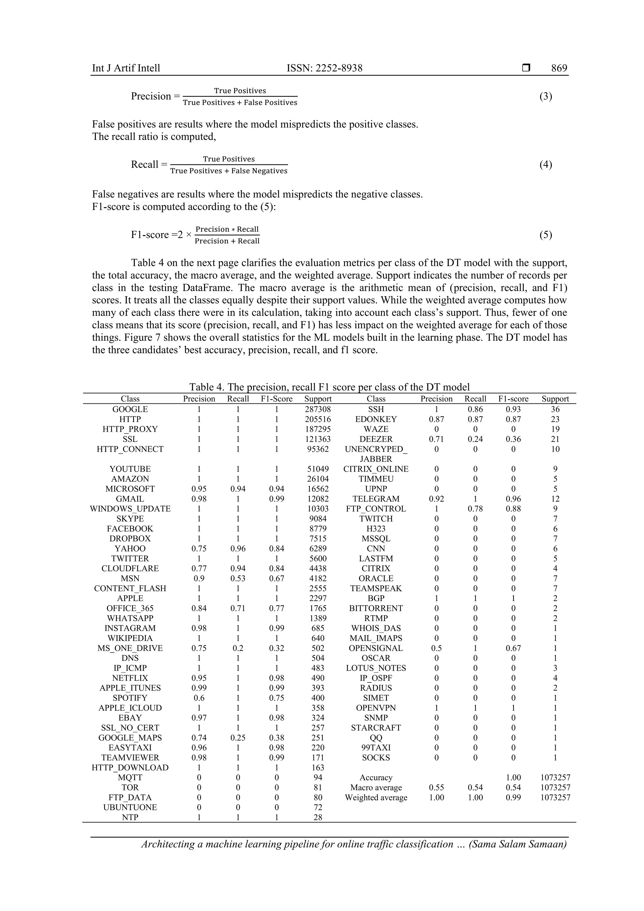
   ISSN: 2252-8938 IntJ Artif Intell, Vol. 12, No. 2, June 2023: 861-873 868 c) Logistic regression Logistic regression (LR) is a predictive analysis, supervised learning algorithm for classifying categorical variables. It is built on the concept of probability. In LR, the output is transformed using the logistic sigmoid function to return a probability value. After all the stages are prepared, they are placed in the pipeline. Using the training DataFrame, the pipeline is fitted to produce the ML models to be evaluated and used in the deployment phase to make predictions. This is illustrated in part (b) of Figure 3. Table 3. The hyperparameter tuning for the machine learning algorithms Model Parameter Explanation Value Decision tree maxDepth The maximum tree depth, the default equals 5 10 impurity The required criterion for the selection of information gain (gini or entropy) gini Logistic regression maxIter max number of iterations 150 family Can be multinomial or binary multinomial standardization Whether to standardize the training features before fitting the model TRUE elasticNetParam A floating-point value from 0 to 1. This parameter specifies the mix of L1 and L2 regularization according to elastic net regularization 0.8 Random forest numTrees The total number of trees to train 200 maxDepth Maximum depth of the tree, must be in range [0, 30] 8 maxBins Max number of bins for discretizing continuous features. Must be >=2 32 4.2. Deployment phase The deployment phase consists of the messaging system, spark streaming, and the ML model. The messaging system is responsible for transmitting traffic data from the SDN controller to spark streaming to perform the required analysis. The chosen messaging system should be scalable, fault-tolerant, elastic, and can transfer high volumes of data in real-time with low latency. Apache Kafka has all these capabilities [32]. In addition, it can be integrated conveniently with open network operating system (ONOS) and opendaylight (ODL) since these controllers have northbound plugins that allow real-time event streaming into Kafka [33], [34]. The SDN controller publishes traffic flow data as messages on Kafka using a common topic. Then, Spark streaming subscribes to that topic and acquires the message streams from Kafka. Spark streaming represents the analytics point that performs data cleaning and preprocessing to generate the required information for the ML model [35]. The ML models built in the learning phase are evaluated in terms of accuracy and speed. Based on the evaluation results, the ML model with the best performance is used in the deployment phase to predict the application class. These predictions are utilized in making management decisions like resource allocation, routing, load balancing, to improve the network performance and lower the time required to detect security threats. The deployment phase implementation is currently beyond the scope of this work. 5. ML MODELS EVALUATION AND TESTING This section evaluates and tests the ML models built in the learning phase. The pipeline implementation, evaluation, and testing are done on a laptop with CPU intel core (TM) i7 and installed memory (RAM) of 16 GB. The software tools are apache spark 3.2.1 and python 3.10. By default, spark driver memory is configured to 1 GB which is insufficient for this work since the training dataset size equals 1.64 GB. So, the amount of memory needed for the driver process is configured to 15 GB to prevent out of memory errors. 5.1. ML models evaluation In this subsection, the accuracy of each ML model is computed. The model with the highest performance will be applied in the deployment phase. Accuracy is calculated according to the following [36], Accuracy = True Positives + True Negatives All Samples (2) True positives, also known as sensitivity, are results where the model predicts the positive classes correctly. True negatives, also known as specificity, are results where the model predicts the negative classes correctly. Besides accuracy, precision, recall, and F1-score metrics are computed because accuracy alone is inadequate to evaluate the performance of the models. The precision ratio outlines the model performance in predicting the positive classes. It is calculated,
• 9.
  Int J ArtifIntell ISSN: 2252-8938  Architecting a machine learning pipeline for online traffic classification … (Sama Salam Samaan) 869 Precision = True Positives True Positives + False Positives (3) False positives are results where the model mispredicts the positive classes. The recall ratio is computed, Recall = True Positives True Positives + False Negatives (4) False negatives are results where the model mispredicts the negative classes. F1-score is computed according to the (5): F1-score =2 × Precision ∗ Recall Precision + Recall (5) Table 4 on the next page clarifies the evaluation metrics per class of the DT model with the support, the total accuracy, the macro average, and the weighted average. Support indicates the number of records per class in the testing DataFrame. The macro average is the arithmetic mean of (precision, recall, and F1) scores. It treats all the classes equally despite their support values. While the weighted average computes how many of each class there were in its calculation, taking into account each class’s support. Thus, fewer of one class means that its score (precision, recall, and F1) has less impact on the weighted average for each of those things. Figure 7 shows the overall statistics for the ML models built in the learning phase. The DT model has the three candidates’ best accuracy, precision, recall, and f1 score. Table 4. The precision, recall F1 score per class of the DT model Class Precision Recall F1-Score Support Class Precision Recall F1-score Support GOOGLE 1 1 1 287308 SSH 1 0.86 0.93 36 HTTP 1 1 1 205516 EDONKEY 0.87 0.87 0.87 23 HTTP_PROXY 1 1 1 187295 WAZE 0 0 0 19 SSL 1 1 1 121363 DEEZER 0.71 0.24 0.36 21 HTTP_CONNECT 1 1 1 95362 UNENCRYPED_ JABBER 0 0 0 10 YOUTUBE 1 1 1 51049 CITRIX_ONLINE 0 0 0 9 AMAZON 1 1 1 26104 TIMMEU 0 0 0 5 MICROSOFT 0.95 0.94 0.94 16562 UPNP 0 0 0 5 GMAIL 0.98 1 0.99 12082 TELEGRAM 0.92 1 0.96 12 WINDOWS_UPDATE 1 1 1 10303 FTP_CONTROL 1 0.78 0.88 9 SKYPE 1 1 1 9084 TWITCH 0 0 0 7 FACEBOOK 1 1 1 8779 H323 0 0 0 6 DROPBOX 1 1 1 7515 MSSQL 0 0 0 7 YAHOO 0.75 0.96 0.84 6289 CNN 0 0 0 6 TWITTER 1 1 1 5600 LASTFM 0 0 0 5 CLOUDFLARE 0.77 0.94 0.84 4438 CITRIX 0 0 0 4 MSN 0.9 0.53 0.67 4182 ORACLE 0 0 0 7 CONTENT_FLASH 1 1 1 2555 TEAMSPEAK 0 0 0 7 APPLE 1 1 1 2297 BGP 1 1 1 2 OFFICE_365 0.84 0.71 0.77 1765 BITTORRENT 0 0 0 2 WHATSAPP 1 1 1 1389 RTMP 0 0 0 2 INSTAGRAM 0.98 1 0.99 685 WHOIS_DAS 0 0 0 1 WIKIPEDIA 1 1 1 640 MAIL_IMAPS 0 0 0 1 MS_ONE_DRIVE 0.75 0.2 0.32 502 OPENSIGNAL 0.5 1 0.67 1 DNS 1 1 1 504 OSCAR 0 0 0 1 IP_ICMP 1 1 1 483 LOTUS_NOTES 0 0 0 3 NETFLIX 0.95 1 0.98 490 IP_OSPF 0 0 0 4 APPLE_ITUNES 0.99 1 0.99 393 RADIUS 0 0 0 2 SPOTIFY 0.6 1 0.75 400 SIMET 0 0 0 1 APPLE_ICLOUD 1 1 1 358 OPENVPN 1 1 1 1 EBAY 0.97 1 0.98 324 SNMP 0 0 0 1 SSL_NO_CERT 1 1 1 257 STARCRAFT 0 0 0 1 GOOGLE_MAPS 0.74 0.25 0.38 251 QQ 0 0 0 1 EASYTAXI 0.96 1 0.98 220 99TAXI 0 0 0 1 TEAMVIEWER 0.98 1 0.99 171 SOCKS 0 0 0 1 HTTP_DOWNLOAD 1 1 1 163 MQTT 0 0 0 94 Accuracy 1.00 1073257 TOR 0 0 0 81 Macro average 0.55 0.54 0.54 1073257 FTP_DATA 0 0 0 80 Weighted average 1.00 1.00 0.99 1073257 UBUNTUONE 0 0 0 72 NTP 1 1 1 28
• 10.
   ISSN: 2252-8938 IntJ Artif Intell, Vol. 12, No. 2, June 2023: 861-873 870 Figure 7. Evaluation metrics for the DT, RF, and LR models 5.2. Comparative analysis A part of the evaluation process is to compare the proposed work with the state-of-the-art. Kuranage et al. [7] is considered for comparison since it used the same dataset [22] for training. To the best of our knowledge, [7] is the only work that used this dataset for SDN traffic classification and prediction. The comparison is fourfold. First, Kuranage et al. [7], did not apply the ML pipeline concept used in this work to automate the ML workflow. Second, Kuranage et al. [7], feature selection was applied manually so that only eight features were used in model building. While in this work, feature selection is applied based on the variance thresholding technique. Ten features are removed utilizing this technique (detailed in subsection 4.1). Third, spark is employed as a big data framework in this work for ML model building using the MLlib library and spark streaming for prototype testing. However, [7] didn’t use any big data tool. Finally, the accuracy of the DT model is 0.98, as indicated in the previous section. In comparison, it was 0.95 Kuranage et al. [7]. 5.3. The prototype testing To test the ML models produced from the learning phase, there is a need to replicate the online data streaming. Therefore, a prototype is implemented in which the testing DataFrame is repartitioned into 1,000 different files; each file has approximately 1,072 records. Generally speaking, spark streaming accepts data from various sources (e.g., file source, Flume, Kafka) and processes it in real-time. Figure 8 illustrates the streaming process from a file directory as a data source for spark streaming. In the implemented prototype, Spark streaming listens to the file directory where the testing files are stored. Since the DT model has the best accuracy among the other models, it is used to predict traffic applications. Figure 9(a) shows life data streaming, where the number of streamed and processed records fluctuates around 300 records per second. This part sets the maximum number of files per trigger to 1. While in Figure 9(b), the number of streamed and processed records is nearly doubled since the maximum number of files per trigger is set to 2. The processing becomes faster since the number of files per trigger is doubled. Figure 8. File source for streaming data to the ML model
• 11.
  Int J ArtifIntell ISSN: 2252-8938  Architecting a machine learning pipeline for online traffic classification … (Sama Salam Samaan) 871 Figure 10 shows a sample snapshot of the streaming, including the actual label, the probability, and the model prediction. As seen in the first row, the vector in the probability column is [1,0,0., 0]. The first value in the vector is the probability of class 0 (Google), the second value is the probability of class 1 (HTTP), and so on. The model chooses the larger probability and designates the streamed data to the class with the larger probability. In the case of the first row, the model selects the larger probability, i.e., 1, and designates the streamed data to class 0 (Google), and it is correct compared with the actual label. In the second row, the model chooses the larger probability, i.e., 0.9923805704546593, and designates the streamed data to class 8 (Gmail), which is correct compared with the actual label. Figure 9. Input vs processing rate (a) max files per trigger = 1 (b) max files per trigger = 2. note: max files per trigger is the maximum number of new files to be processed in every trigger. Figure 10. Sample output of the label, probability, and prediction on the unseen data 6. CONCLUSION This paper presented the architecture of a ML pipeline for online SDN network traffic classification using spark. The proposed model consists of two phases; learning and deployment. A pipeline is designed to streamline and automate the ML processes in the learning phase. Three ML models are built using the Spark ML library; decision tree, random forest, and logistic regression. These models are evaluated in four terms of evaluation metrics; accuracy, precision, recall, and f1-score. Results show that the decision tree model has the best accuracy with 0.98. Spark streaming is incorporated to stream the data to the elected ML model to replicate the online network traffic flow of data. In future work, the second phase of the proposed model, i.e., deployment, is intended to be implemented to utilize the valuable information acquired from the learning phase in diverse network management aspects, including routing, load balancing, and resource allocation. REFERENCES [1] L.-V. Le, B.-S. Lin, and S. Do, “Applying big data, machine learning, and SDN/NFV for 5G early-stage traffic classification and network QoS control,” Transactions on Networks and Communications, vol. 6, no. 2, Apr. 2018, doi: 10.14738/tnc.62.4446. [2] R. M. AlZoman and M. J. F. Alenazi, “A comparative study of traffic classification techniques for smart city networks,” Sensors, vol. 21, no. 14, p. 4677, Jul. 2021, doi: 10.3390/s21144677.
• 12.
   ISSN: 2252-8938 IntJ Artif Intell, Vol. 12, No. 2, June 2023: 861-873 872 [3] A. A. Ahmed and G. Agunsoye, “A real-time network traffic classifier for online applications using machine learning,” Algorithms, vol. 14, no. 8, p. 250, Aug. 2021, doi: 10.3390/a14080250. [4] M. A. Ridwan, N. A. M. Radzi, F. Abdullah, and Y. E. Jalil, “Applications of machine learning in networking: a survey of current issues and future challenges,” IEEE Access, vol. 9, pp. 52523–52556, 2021, doi: 10.1109/ACCESS.2021.3069210. [5] Imran, Z. Ghaffar, A. Alshahrani, M. Fayaz, A. M. Alghamdi, and J. Gwak, “A topical review on machine learning, software defined networking, internet of things applications: research limitations and challenges,” Electronics, vol. 10, no. 8, p. 880, Apr. 2021, doi: 10.3390/electronics10080880. [6] A. S. Dawood and M. N. Abdullah, “Adaptive performance evaluation for SDN based on the statistical and evolutionary algorithms,” Iraqi Journal of Computer, Communication, Control and System Engineering, pp. 36–46, Oct. 2019, doi: 10.33103/uot.ijccce.19.4.5. [7] M. P. J. Kuranage, K. Piamrat, and S. Hamma, “Network traffic classification using machine learning for software defined networks,” in IFIP International Conference on Machine Learning for Networking (MLN’2019), 2020, pp. 28–39. [8] M. Reza, M. Javad, S. Raouf, and R. Javidan, “Network traffic classification using machine learning techniques over software defined networks,” International Journal of Advanced Computer Science and Applications, vol. 8, no. 7, 2017, doi: 10.14569/IJACSA.2017.080729. [9] M. M. Raikar, M. S M, M. M. Mulla, N. S. Shetti, and M. Karanandi, “Data traffic classification in software defined networks (SDN) using supervised-learning,” Procedia Computer Science, vol. 171, pp. 2750–2759, 2020, doi: 10.1016/j.procs.2020.04.299. [10] A. I. Owusu and A. Nayak, “An intelligent traffic classification in SDN-IoT: a machine learning approach,” in 2020 IEEE International Black Sea Conference on Communications and Networking (BlackSeaCom), May 2020, pp. 1–6, doi: 10.1109/BlackSeaCom48709.2020.9235019. [11] A. Malik, R. de Frein, M. Al-Zeyadi, and J. Andreu-Perez, “Intelligent SDN traffic classification using deep learning: deep- SDN,” in 2020 2nd International Conference on Computer Communication and the Internet (ICCCI), Jun. 2020, pp. 184–189, doi: 10.1109/ICCCI49374.2020.9145971. [12] L.-H. Chang, Tsung-Han Lee, Hung-Chi Chu, and Cheng-Wei Su, “Application based online traffic classification with deep learning models on SDN networks,” Advances in Technology Innovation, Jul. 2020, doi: 10.46604/aiti.2020.4286. [13] S. M. Othman, F. M. Ba-Alwi, N. T. Alsohybe, and A. Y. Al-Hashida, “Intrusion detection model using machine learning algorithm on big data environment,” Journal of Big Data, vol. 5, no. 1, p. 34, Dec. 2018, doi: 10.1186/s40537-018-0145-4. [14] M. Belouch, S. El Hadaj, and M. Idhammad, “Performance evaluation of intrusion detection based on machine learning using Apache Spark,” Procedia Computer Science, vol. 127, pp. 1–6, 2018, doi: 10.1016/j.procs.2018.01.091. [15] I. Sassi, S. Anter, and A. Bekkhoucha, “A spark-based parallel distributed posterior decoding algorithm for big data hidden Markov models decoding problem,” IAES International Journal of Artificial Intelligence (IJ-AI), vol. 10, no. 3, p. 789, Sep. 2021, doi: 10.11591/ijai.v10.i3.pp789-800. [16] A. Mostafaeipour, A. Jahangard Rafsanjani, M. Ahmadi, and J. Arockia Dhanraj, “Investigating the performance of Hadoop and Spark platforms on machine learning algorithms,” The Journal of Supercomputing, vol. 77, no. 2, pp. 1273–1300, Feb. 2021, doi: 10.1007/s11227-020-03328-5. [17] A. Mahmood and A. Kareem, “A new processing approach for scheduling time minimization in 5G-IoT networks,” International Journal of Intelligent Engineering and Systems, vol. 14, no. 3, pp. 481–492, Jun. 2021, doi: 10.22266/ijies2021.0630.40. [18] V. Abeykoon et al., “Streaming machine learning algorithms with big data systems,” in 2019 IEEE International Conference on Big Data (Big Data), Dec. 2019, pp. 5661–5666, doi: 10.1109/BigData47090.2019.9006337. [19] R. Karsi, M. Zaim, and J. El Alami, “Assessing naive bayes and support vector machine performance in sentiment classification on a big data platform,” IAES International Journal of Artificial Intelligence (IJ-AI), vol. 10, no. 4, p. 990, Dec. 2021, doi: 10.11591/ijai.v10.i4.pp990-996. [20] “Spark machine learning library (MLlib) guide,” Apache Spark. https://spark.apache.org/docs/latest/ml-guide.html (accessed Mar. 10, 2022). [21] S. Wang, J. Luo, and L. Luo, “Large-scale text multiclass classification using spark ML packages,” Journal of Physics: Conference Series, vol. 2171, no. 1, p. 12022, Jan. 2022, doi: 10.1088/1742-6596/2171/1/012022. [22] J. S. Rojas, “IP network traffic flows labeled with 75 apps,” Kaggle, 2018. https://www.kaggle.com/datasets/jsrojas/ip-network- traffic-flows-labeled-with-87-apps (accessed Mar. 10, 2022). [23] J. S. Rojas, Á. R. Gallón, and J. C. Corrales, “Personalized service degradation policies on OTT applications based on the consumption behavior of users,” 2018, pp. 543–557. [24] F. Pacheco, E. Exposito, M. Gineste, C. Baudoin, and J. Aguilar, “Towards the deployment of machine learning solutions in network traffic classification: a systematic survey,” IEEE Communications Surveys & Tutorials, vol. 21, no. 2, pp. 1988–2014, 2019, doi: 10.1109/COMST.2018.2883147. [25] “Spark documentation,” Apache Spark, 2018. https://spark.apache.org/docs/3.2.1/index.html (accessed Jan. 10, 2022). [26] S. D. Khudhur and H. A. Jeiad, “A content-based file identification dataset: collection, construction, and evaluation,” Karbala International Journal of Modern Science, vol. 8, no. 2, pp. 63–70, May 2022, doi: 10.33640/2405-609X.3222. [27] A. A. Afuwape, Y. Xu, J. H. Anajemba, and G. Srivastava, “Performance evaluation of secured network traffic classification using a machine learning approach,” Computer Standards & Interfaces, vol. 78, p. 103545, Oct. 2021, doi: 10.1016/j.csi.2021.103545. [28] J. Xie et al., “A survey of machine learning techniques applied to software defined networking (SDN): research issues and challenges,” IEEE Communications Surveys & Tutorials, vol. 21, no. 1, pp. 393–430, 2019, doi: 10.1109/COMST.2018.2866942. [29] N. N. Qomariyah, E. Heriyanni, A. N. Fajar, and D. Kazakov, “Comparative analysis of decision tree algorithm for learning ordinal data expressed as pairwise comparisons,” in 2020 8th International Conference on Information and Communication Technology (ICoICT), Jun. 2020, pp. 1–4, doi: 10.1109/ICoICT49345.2020.9166341. [30] H. AL-Behadili, “Decision tree for multiclass classification of firewall access,” International Journal of Intelligent Engineering and Systems, vol. 14, no. 3, pp. 294–302, Jun. 2021, doi: 10.22266/ijies2021.0630.25. [31] Y. Xiao, W. Huang, and J. Wang, “A random forest classification algorithm based on dichotomy rule fusion,” in 2020 IEEE 10th International Conference on Electronics Information and Emergency Communication (ICEIEC), Jul. 2020, pp. 182–185, doi: 10.1109/ICEIEC49280.2020.9152236. [32] B. Zhou et al., “Online internet traffic monitoring system using spark streaming,” Big Data Mining and Analytics, vol. 1, no. 1, pp. 47–56, Mar. 2018, doi: 10.26599/BDMA.2018.9020005. [33] “Opendaylight (ODL),” open Daylight, 2021. https://www.opendaylight.org/ (accessed Feb. 03, 2022). [34] “Open network operating system (ONOS),” ONOS, 2020. https://wiki.onosproject.org/ (accessed Jan. 03, 2022). [35] B. Zhou, J. Li, J. Wu, S. Guo, Y. Gu, and Z. Li, “Machine-learning-based online distributed denial-of-service attack detection
• 13.
  Int J ArtifIntell ISSN: 2252-8938  Architecting a machine learning pipeline for online traffic classification … (Sama Salam Samaan) 873 using spark streaming,” in 2018 IEEE International Conference on Communications (ICC), May 2018, pp. 1–6, doi: 10.1109/ICC.2018.8422327. [36] O. Jonathan, S. Misra, and V. Osamor, “Comparative analysis of machine learning techniques for network traffic classification,” IOP Conference Series: Earth and Environmental Science, vol. 655, no. 1, p. 12025, Feb. 2021, doi: 10.1088/1755- 1315/655/1/012025. BIOGRAPHIES OF AUTHORS Sama Salam Samaan is currently a PhD student and lecturer in the Computer Engineering Department at the University of Technology in Baghdad, Iraq. She received her undergraduate degree in Information Engineering from this department in 2005. In 2011, she earned her Master’s Degree from Al-Nahrain University in Baghdad, Iraq. She published several papers in national journals, including Al-Nahrain Journal for Engineering Sciences, Al-Khwarizmi Engineering Journal, The Journal of Engineering, and Journal of Engineering and Sustainable Development. Her research activities concern big data, software defined networks (SDN), and machine learning. She can be contacted at email: sama.s.samaan@uotechnology.edu.iq. Dr Hassan Awheed Jeiad Received a B.Sc. degree in 1989 in Electronics and Communications Engineering from the University of Technology, Baghdad, Iraq. He received his Master’s Degree in Communication Engineering from the University of Technology, Baghdad, Iraq, in 1999. Dr Hassan received his PhD in Computer Engineering in 2006 from the University of Technology, Baghdad, Iraq. Currently, he is an assistant professor in the Department of Computer Engineering at the University of Technology, Baghdad, Iraq. His research interests include computer architecture, microprocessors, computer networks, multimedia, adaptive systems, and information systems. He can be contacted at email: hassan.a.jeiad@uotechnology.edu.iq.