IJESM Volume 2, Issue 3 ISSN: 2320-0294 _________________________________________________________ A Quarterly Double-Blind Peer Reviewed Refereed Open Access International e-Journal - Included in the International Serial Directories Indexed & Listed at: Ulrich's Periodicals Directory ©, U.S.A., Open J-Gage, India as well as in Cabell’s Directories of Publishing Opportunities, U.S.A. International Journal of Engineering, Science and Mathematics http://www.ijmra.us 107 September 2013 APPLICATION OF THE METHOD OF VARIATION OF PARAMETERS: MATHEMATICAL MODEL FOR DEVELOPING AND ANALYZING STABILITY OF THE WAGE FUNCTION Olala, Gilbert Owuor Abstract In this paper, a second order wage equation is developed and solved by the method of variation of parameters. The subsequent wage function is then analyzed and interpreted for stability. Speculative parameters, which operate freely dictating employers’ expectations, are included in modeling this equation. The variation of these parameters causes both stability and instability of the wage function depending on circumstances. Where the wage function is exponential, asymptotic stability towards the equilibrium wage rate is observed but where it consists of both exponential and periodic factors, the time path shows periodic fluctuations with successive cycles giving smaller amplitudes until the ripples die naturally. It has been realized that where the wage rate is determined by free market forces of demand and supply, volatility in wage rate may be observed if not controlled. This may increase uncertainties and cause anxiety about investment and employment in the economy. The paper therefore proposes government intervention by creating a middle path in which wage rate is allowed to oscillate freely within a narrow band managed by employers in consultation with the workers under the watch of the government. Key words: wage equation, wage function, wage rate, equilibrium wage rate, stability, market forces, volatile wage rate, and middle path.  Department of Mathematics & Computer Science, Kisumu Polytechnic, Kisumu, KENYA
IJESM Volume 2, Issue 3 ISSN: 2320-0294 _________________________________________________________ A Quarterly Double-Blind Peer Reviewed Refereed Open Access International e-Journal - Included in the International Serial Directories Indexed & Listed at: Ulrich's Periodicals Directory ©, U.S.A., Open J-Gage, India as well as in Cabell’s Directories of Publishing Opportunities, U.S.A. International Journal of Engineering, Science and Mathematics http://www.ijmra.us 108 September 2013 1. Introduction Wages mean the reward for labor services. In [6] wage is defined as a fixed regular payment earned for work or services, typically paid on a daily or weekly basis. In [9] wage is viewed as payment for labour services to a worker, especially remuneration on an hourly, daily, weekly or by piece. It also views wage as a portion of national product that represents aggregate paid for all contributing labour and services as distinguished from the portion retained by management or reinvested in capital goods. In [10] wage is defined according to wages act of 1986. It is the sum payable to an employee by an employer in connection with that employment. It includes fees, bonuses, commissions, holiday pay or other emolument relevant to the employment whether specified in the contract of employment or not. In this paper, we consider modeling a second order differential wage equation. For example, considering deterministic price adjustment model in [7] fixed supply and demand functions at instantaneous price for security is discussed. It is argued that at equilibrium asset price, quantity demanded equals quantity supplied. This is discussed using fixed demand and supply curves while price is kept constant. It also asserts that away from the equilibrium, excess demand for security raises its price, and excess supply lowers its price. In this situation, it is argued that the sign for rate of change of price with respect to time depends on the sign of excess demand. If the demand and supply functions are made linear at constant equilibrium price, deterministic model of price adjustment is realized with respective sensitivities. In the analysis of the solution of the deterministic model, it was observed that in the long run asset price settles at a constant steady state where no further change can occur. In [4] a natural decay equation is developed. The equation describes a phenomenon where a quantity gradually decreases to zero. In the work, it is emphasized that convergence depends the sign of the proportionality parameter. If the proportionality parameter is negative then it turns into a growth equation but if it is positive, it stabilizes in the long run. In the study of slope fields for autonomous equations qualitative properties of decay equation is demonstrated. It was found that the solution could be positive, negative or zero. In all the three cases, the solution approaches zero in limit as time approaches infinity.
IJESM Volume 2, Issue 3 ISSN: 2320-0294 _________________________________________________________ A Quarterly Double-Blind Peer Reviewed Refereed Open Access International e-Journal - Included in the International Serial Directories Indexed & Listed at: Ulrich's Periodicals Directory ©, U.S.A., Open J-Gage, India as well as in Cabell’s Directories of Publishing Opportunities, U.S.A. International Journal of Engineering, Science and Mathematics http://www.ijmra.us 109 September 2013 In [1], dynamics of market prices are studied. It was found out that if the initial price function lies off the equilibrium point, in the long run stability will be realized at the equilibrium position. It also brings out clear case by case analysis of the solution of second order price equation by introducing unrestricted parameters that brings speculations in behavior of buyers and sellers. The author argued that depending on the signs of these parameters, buyers will cut or increase their purchases. Similarly, sellers will cut or increase their supplies. It was also noted that depending on signs of parameters, price function stabilizes in the long run. In [2], equilibrium solutions about a special class of static solutions are discussed. The study found that if a system starts exactly at equilibrium position, then it remains there forever. The study further found that in real systems, small disturbances often a rise which moves a system away from equilibrium state. Such disturbances, regardless of their origin give rise to initial conditions which do not coincide with equilibrium condition. If the system is not at equilibrium point, then some of its derivatives will be non zero and the system therefore exhibits a dynamic behavior, which can be monitored by watching orbits in its phase space. The resistance-inductance electric current circuit for constant electromotive force is modeled into a differential equation in [3].The stability of the solution is studied in the long run and is found to be a constant, which is the ratio of constant electromotive force to resistance. It was also found that if electromotive force is periodic, in the long run, current executes harmonic oscillations. In this case, steady state solution is the periodic part of the solution. The resistance-capacitor electric current circuit equation is also discussed for constant electromotive force. The solution was an exponential function, which converges to zero in the long run. Also, in resistance- inductance-capacitance series circuit, a second order equation was developed. Its solution consists of an exponential homogeneous part and a periodic integral part. The study found out that the homogeneous part converges to zero as time approaches infinity, while the periodic part exhibits practically harmonic oscillations. The literature is silent and it is worthwhile developing a second order wage equation, solve it and discuss its stability. The solutions of linear second order ordinary differential equations are presented in [5; 8] using the method of variation of parameters.
IJESM Volume 2, Issue 3 ISSN: 2320-0294 _________________________________________________________ A Quarterly Double-Blind Peer Reviewed Refereed Open Access International e-Journal - Included in the International Serial Directories Indexed & Listed at: Ulrich's Periodicals Directory ©, U.S.A., Open J-Gage, India as well as in Cabell’s Directories of Publishing Opportunities, U.S.A. International Journal of Engineering, Science and Mathematics http://www.ijmra.us 110 September 2013 2. Modeling second order wage equation In this section, we consider modeling a second order linear differential wage equation. In this case, the number demanded and supplied of labor is taken as functions both current wage rate and wage trend prevailing in the market at that time. This is because wage trend will guide laborers expectations regarding future wage level. The expectations will also influence labor demand and supply for future decision making. To include wage trend and expectations, we include continuous time derivatives in the model, i.e. dt dW (2.1) and 2 2 dt Wd (2.2) The derivative (2.1) shows whether the wage function is rising, and the derivative (2.2) shows whether it is rising at an increasing rate. If we consider wage trends, derivatives as additional arguments to labor demand and supply are taken into account. The demand and supply functions are thus given as        2 2 ,),( dt Wd dt dW tWfNd (2.3) and        2 2 ,),( dt Wd dt dW tWfNs (2.4) respectively. Suppose the demand and supply functions of labor are linear, then they are  0,,2 2   dt Wd dt dW WNd (2.5) and  0,,2 2   dt Wd dt dW WNs (2.6) respectively. The other parameters  and,, introduced to dictate employers and laborers expectations have their signs operating in free range. For example, if 0 , a rising wage rate causes the number of laborers demanded to increase. This suggest that employers expect rising wage rate to continue to rise and prefer to increase employment now when the
IJESM Volume 2, Issue 3 ISSN: 2320-0294 _________________________________________________________ A Quarterly Double-Blind Peer Reviewed Refereed Open Access International e-Journal - Included in the International Serial Directories Indexed & Listed at: Ulrich's Periodicals Directory ©, U.S.A., Open J-Gage, India as well as in Cabell’s Directories of Publishing Opportunities, U.S.A. International Journal of Engineering, Science and Mathematics http://www.ijmra.us 111 September 2013 wage rate is still relatively low. On the other hand, for 0 , the wage trend will be falling, and employers will opt to cut current employment while waiting for wage rate to fall even further. The inclusion of the parameter  makes employers behavior to depend also on the rate of change of wage rate dt dW . Thus introducing new parameters  and injects wage rate speculation in the model. Similarly, if we let 0 , then a rising wage rate causes the number of laborers supplied to fall and thus laborers expect the rising wage rate to continue rising and prefer to withhold their services now while waiting for the higher wage rate. On the other hand, for 0 , wage rate will shows a falling trend and laborers will prefer to offer their services now while the wage rate is still relatively high hoping that any delay will see the wage rate fall even further. Therefore, introduction of the parameter  makes the behavior of laborers to depend much on the wage rate just as the employers. We now resort to demonstrating an implicit model by assuming that only labor demand function contains the wage expectations. Specifically, we set both  and of function (2.6) equal to zero; while  and of function (2.5) are set as non zero. Further, we assume that labor market clears at every point in time. We then set the number of laborers demanded equal to the number of laborers supplied to obtain equation bWa dt dW a dt Wd  212 2 (2.7) with                      bandaa ,, 21 , and this is the required second order linear ordinary differential wage equation. 3. Solution of the differential equation In this section, we demonstrate the solution of the differential equation (2.7) using the method of variation of parameters. We first solve equation (2.7) for a complementary solution by considering its homogeneous equation 0212 2  Wa dt dW a dt Wd . (3.1) The characteristic equation of equation (3.1) is
IJESM Volume 2, Issue 3 ISSN: 2320-0294 _________________________________________________________ A Quarterly Double-Blind Peer Reviewed Refereed Open Access International e-Journal - Included in the International Serial Directories Indexed & Listed at: Ulrich's Periodicals Directory ©, U.S.A., Open J-Gage, India as well as in Cabell’s Directories of Publishing Opportunities, U.S.A. International Journal of Engineering, Science and Mathematics http://www.ijmra.us 112 September 2013 021 2  arar . (3.2) Equation (3.2) is quadratic in nature and can be solved for r using the quadratic formula. The roots are therefore given as 2 4 , 2 2 11 21 aaa rr   . (3.3) If we substitute back the values of 21 aanda as given in equation (2.7) the roots become                             4 2 1 , 2 21 rr . (3.4) The roots (3.4) yields varied results depending on the value of the discriminant                  4 2 . This is discussed in three cases. Case I: Suppose 04 2                  then roots 21 randr of the characteristic equation (3.2) are real and different. The complementary solution therefore becomes trctrctWc 2211 expexp)(  (3.5) Case II: Suppose 04 2                  then the roots 21 randr of the characteristic equation (3.2) are real and equal; that is,    2 , 21 rr (3.6) and the complementary solution then becomes   ttcctWc exp)( 21  . (3.7) Case III: Suppose 04 2                  then the roots 21 randr of the characteristic equation (3.2) are complex; that is,  irr 21, ,    2 with and                    4 2 1 2 (3.8) and the complementary solution therefore becomes
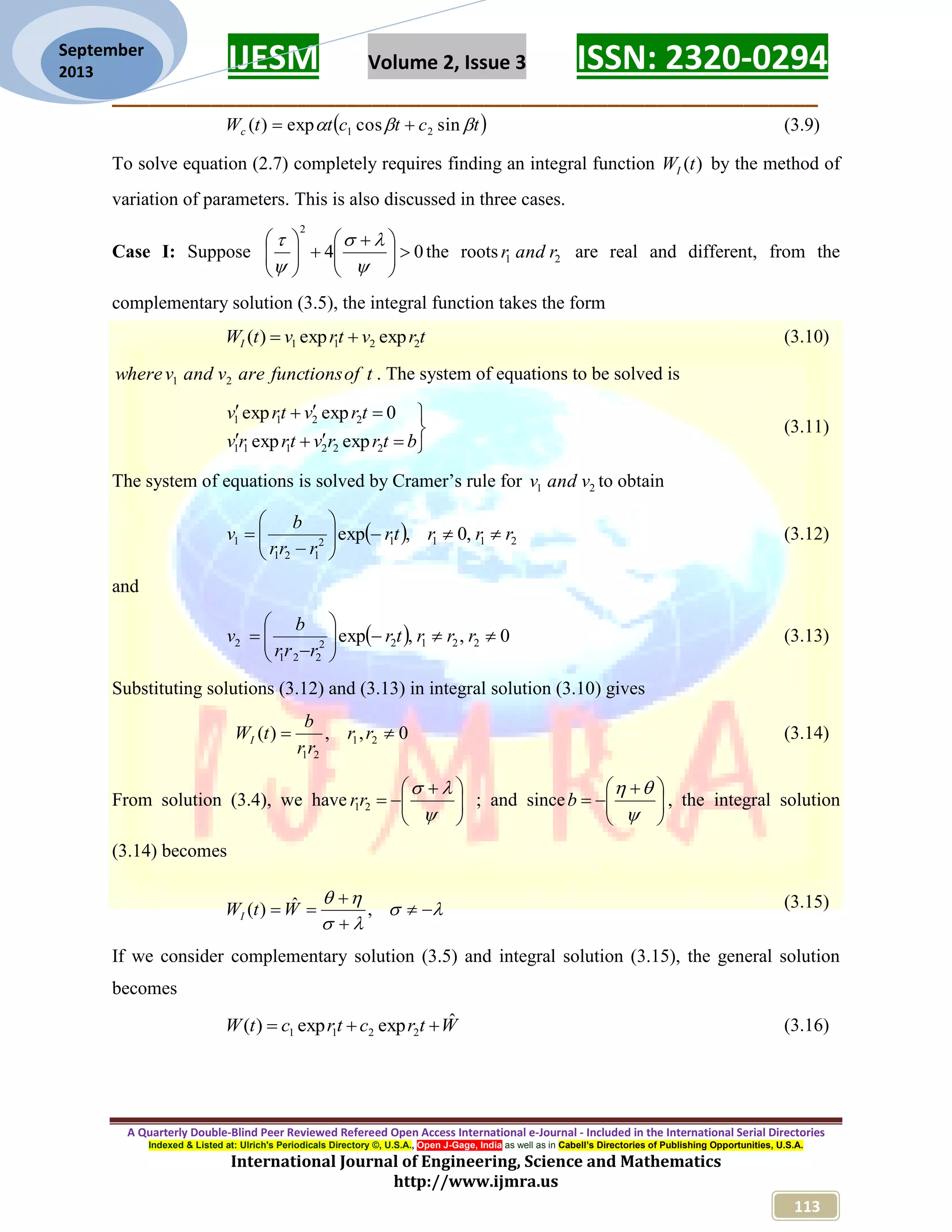
IJESM Volume 2, Issue 3 ISSN: 2320-0294 _________________________________________________________ A Quarterly Double-Blind Peer Reviewed Refereed Open Access International e-Journal - Included in the International Serial Directories Indexed & Listed at: Ulrich's Periodicals Directory ©, U.S.A., Open J-Gage, India as well as in Cabell’s Directories of Publishing Opportunities, U.S.A. International Journal of Engineering, Science and Mathematics http://www.ijmra.us 113 September 2013  tctcttWc  sincosexp)( 21  (3.9) To solve equation (2.7) completely requires finding an integral function )(tWI by the method of variation of parameters. This is also discussed in three cases. Case I: Suppose 04 2                  the roots 21 randr are real and different, from the complementary solution (3.5), the integral function takes the form trvtrvtWI 2211 expexp)(  (3.10) toffunctionsarevandvwhere 21 . The system of equations to be solved is      btrrvtrrv trvtrv 222111 2211 expexp 0expexp (3.11) The system of equations is solved by Cramer’s rule for 21 vandv to obtain   21112 121 1 ,0,exp rrrtr rrr b v         (3.12) and   0,,exp 22122 221 2         rrrtr rrr b v (3.13) Substituting solutions (3.12) and (3.13) in integral solution (3.10) gives 0,,)( 21 21  rr rr b tWI (3.14) From solution (3.4), we have           21rr ; and since           b , the integral solution (3.14) becomes        ,ˆ)( WtWI (3.15) If we consider complementary solution (3.5) and integral solution (3.15), the general solution becomes WtrctrctW ˆexpexp)( 2211  (3.16)
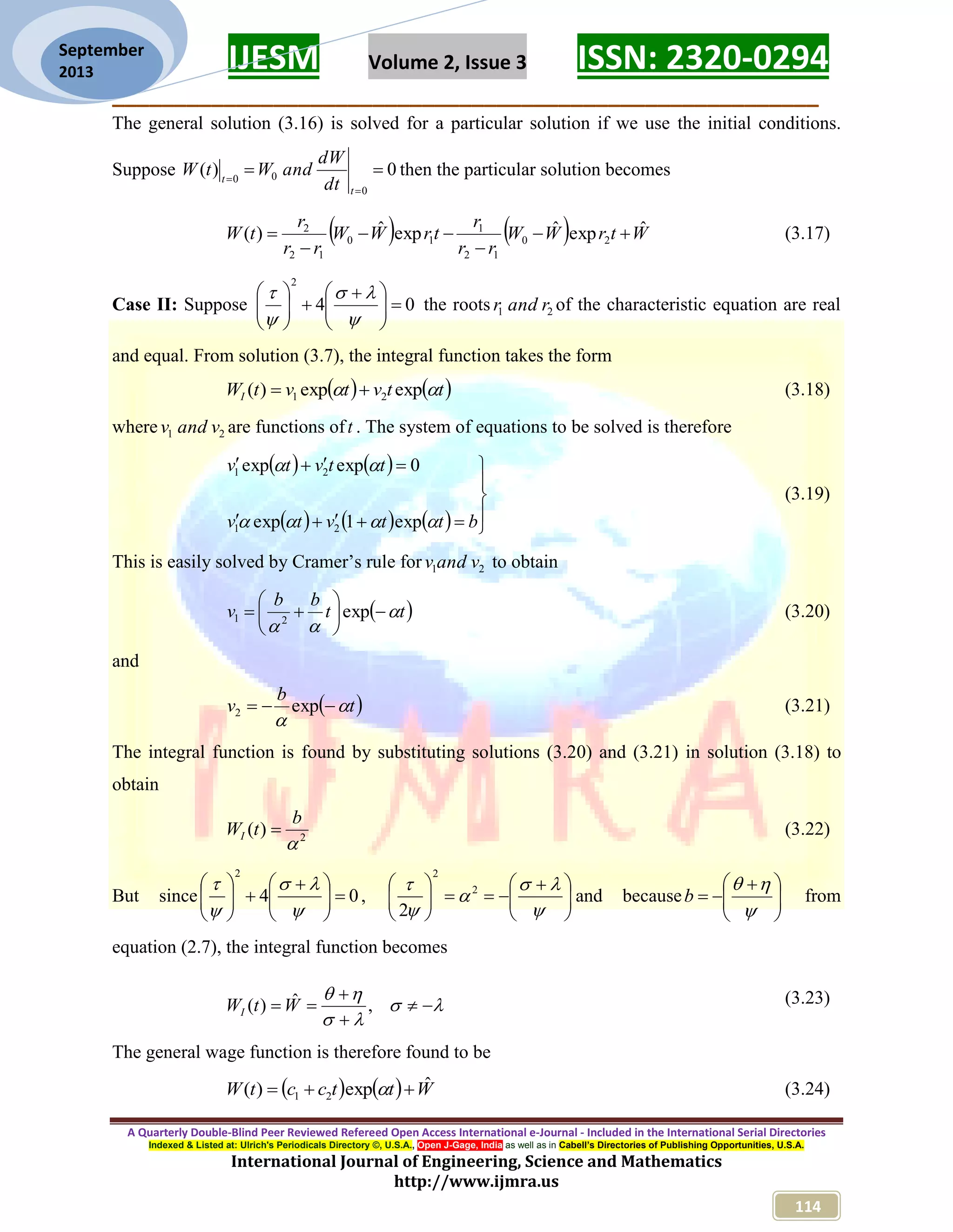
IJESM Volume 2, Issue 3 ISSN: 2320-0294 _________________________________________________________ A Quarterly Double-Blind Peer Reviewed Refereed Open Access International e-Journal - Included in the International Serial Directories Indexed & Listed at: Ulrich's Periodicals Directory ©, U.S.A., Open J-Gage, India as well as in Cabell’s Directories of Publishing Opportunities, U.S.A. International Journal of Engineering, Science and Mathematics http://www.ijmra.us 114 September 2013 The general solution (3.16) is solved for a particular solution if we use the initial conditions. Suppose 0)( 0 00    t t dt dW andWtW then the particular solution becomes     WtrWW rr r trWW rr r tW ˆexpˆexpˆ)( 20 12 1 10 12 2      (3.17) Case II: Suppose 04 2                  the roots 21 randr of the characteristic equation are real and equal. From solution (3.7), the integral function takes the form    ttvtvtWI  expexp)( 21  (3.18) where 21 vandv are functions oft . The system of equations to be solved is therefore                  bttvtv ttvtv   exp1exp 0expexp 21 21 (3.19) This is easily solved by Cramer’s rule for 21 vandv to obtain  tt bb v          exp21 (3.20) and  t b v    exp2 (3.21) The integral function is found by substituting solutions (3.20) and (3.21) in solution (3.18) to obtain 2 )(  b tWI  (3.22) But since 04 2                  ,                   2 2 2 and because           b from equation (2.7), the integral function becomes        ,ˆ)( WtWI (3.23) The general wage function is therefore found to be     WttcctW ˆexp)( 21   (3.24)
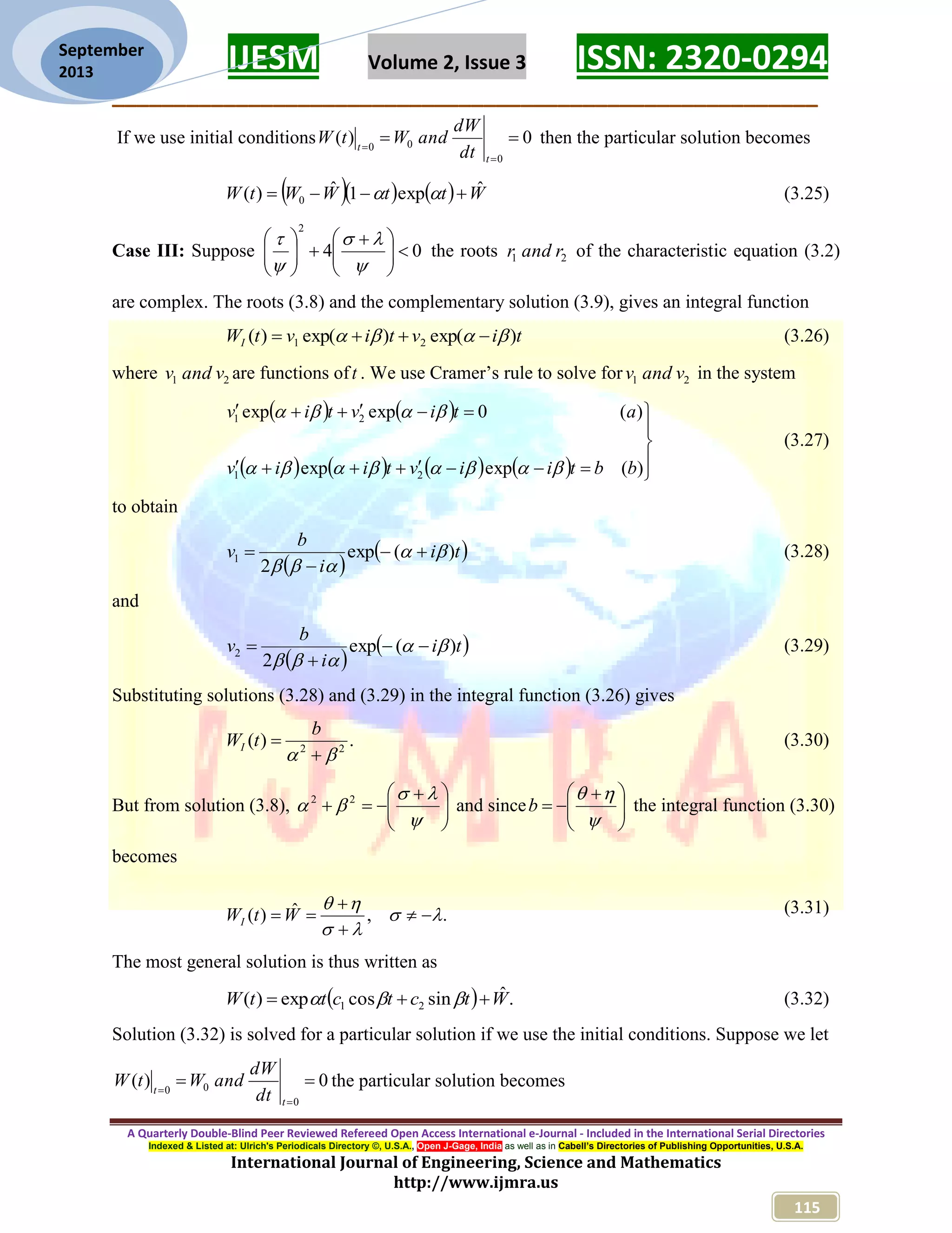
IJESM Volume 2, Issue 3 ISSN: 2320-0294 _________________________________________________________ A Quarterly Double-Blind Peer Reviewed Refereed Open Access International e-Journal - Included in the International Serial Directories Indexed & Listed at: Ulrich's Periodicals Directory ©, U.S.A., Open J-Gage, India as well as in Cabell’s Directories of Publishing Opportunities, U.S.A. International Journal of Engineering, Science and Mathematics http://www.ijmra.us 115 September 2013 If we use initial conditions 0)( 0 00    t t dt dW andWtW then the particular solution becomes      WttWWtW ˆexp1ˆ)( 0   (3.25) Case III: Suppose 04 2                  the roots 21 randr of the characteristic equation (3.2) are complex. The roots (3.8) and the complementary solution (3.9), gives an integral function tivtivtWI )exp()exp()( 21   (3.26) where 21 vandv are functions oft . We use Cramer’s rule to solve for 21 vandv in the system                    )(expexp )(0expexp 21 21 bbtiivtiiv ativtiv   (3.27) to obtain    ti i b v )(exp 2 1      (3.28) and    ti i b v )(exp 2 2      (3.29) Substituting solutions (3.28) and (3.29) in the integral function (3.26) gives .)( 22    b tWI (3.30) But from solution (3.8),            22 and since           b the integral function (3.30) becomes .,ˆ)(       WtWI (3.31) The most general solution is thus written as   .ˆsincosexp)( 21 WtctcttW   (3.32) Solution (3.32) is solved for a particular solution if we use the initial conditions. Suppose we let 0)( 0 00    t t dt dW andWtW the particular solution becomes
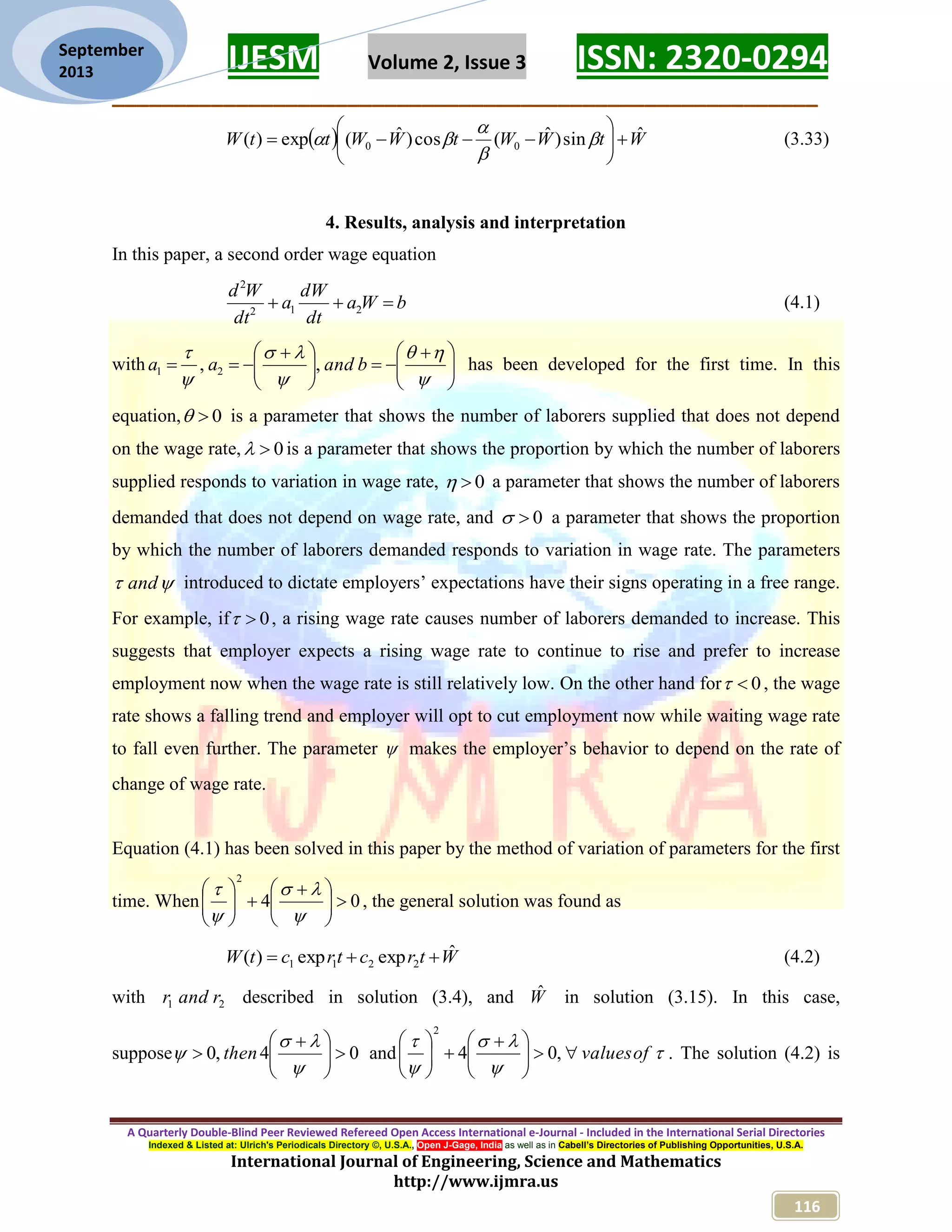
IJESM Volume 2, Issue 3 ISSN: 2320-0294 _________________________________________________________ A Quarterly Double-Blind Peer Reviewed Refereed Open Access International e-Journal - Included in the International Serial Directories Indexed & Listed at: Ulrich's Periodicals Directory ©, U.S.A., Open J-Gage, India as well as in Cabell’s Directories of Publishing Opportunities, U.S.A. International Journal of Engineering, Science and Mathematics http://www.ijmra.us 116 September 2013   WtWWtWWttW ˆsin)ˆ(cos)ˆ(exp)( 00            (3.33) 4. Results, analysis and interpretation In this paper, a second order wage equation bWa dt dW a dt Wd  212 2 (4.1) with                      bandaa ,, 21 has been developed for the first time. In this equation, 0 is a parameter that shows the number of laborers supplied that does not depend on the wage rate, 0 is a parameter that shows the proportion by which the number of laborers supplied responds to variation in wage rate, 0 a parameter that shows the number of laborers demanded that does not depend on wage rate, and 0 a parameter that shows the proportion by which the number of laborers demanded responds to variation in wage rate. The parameters  and introduced to dictate employers’ expectations have their signs operating in a free range. For example, if 0 , a rising wage rate causes number of laborers demanded to increase. This suggests that employer expects a rising wage rate to continue to rise and prefer to increase employment now when the wage rate is still relatively low. On the other hand for 0 , the wage rate shows a falling trend and employer will opt to cut employment now while waiting wage rate to fall even further. The parameter  makes the employer’s behavior to depend on the rate of change of wage rate. Equation (4.1) has been solved in this paper by the method of variation of parameters for the first time. When 04 2                  , the general solution was found as WtrctrctW ˆexpexp)( 2211  (4.2) with 21 randr described in solution (3.4), and Wˆ in solution (3.15). In this case, suppose 04,0            then and      ofvalues             ,04 2 . The solution (4.2) is
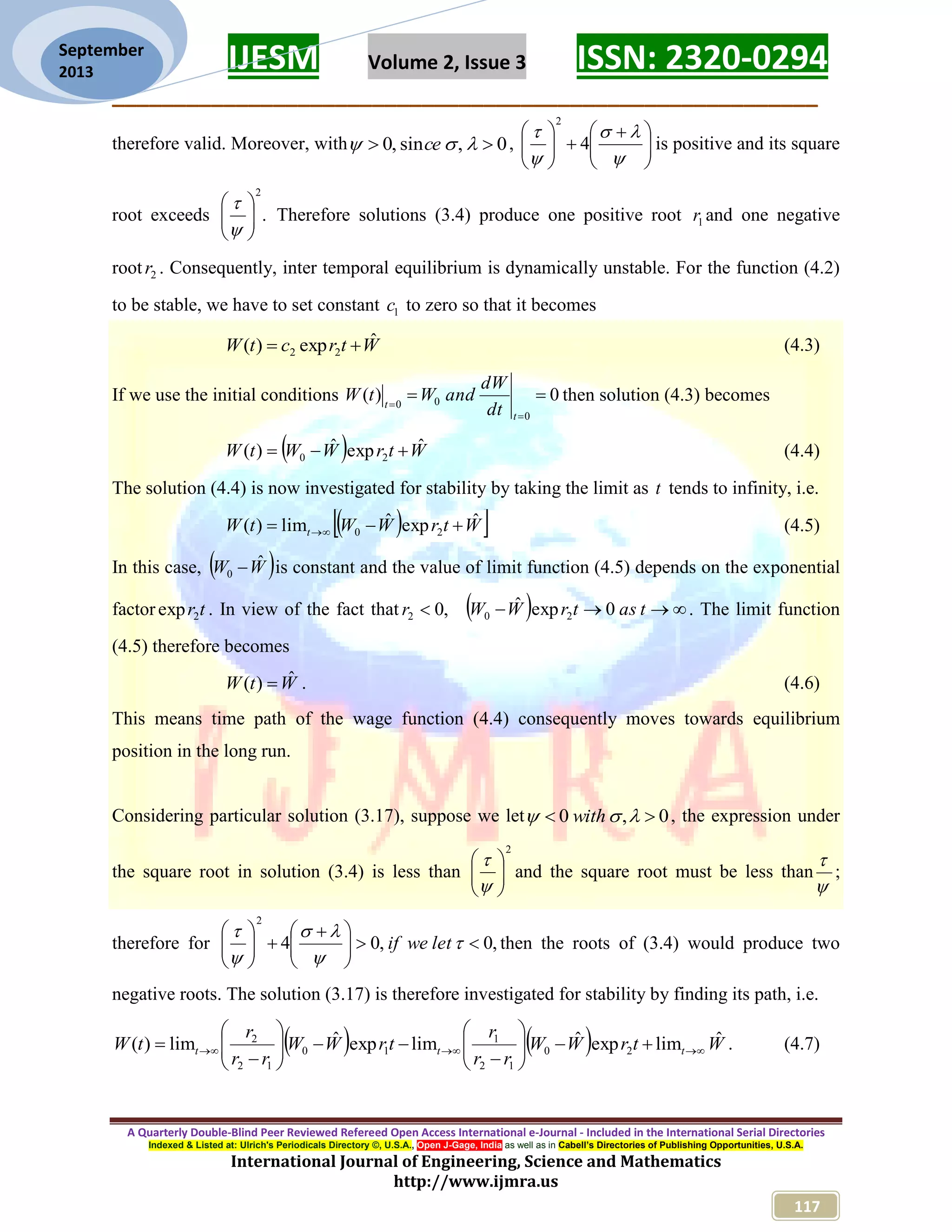
IJESM Volume 2, Issue 3 ISSN: 2320-0294 _________________________________________________________ A Quarterly Double-Blind Peer Reviewed Refereed Open Access International e-Journal - Included in the International Serial Directories Indexed & Listed at: Ulrich's Periodicals Directory ©, U.S.A., Open J-Gage, India as well as in Cabell’s Directories of Publishing Opportunities, U.S.A. International Journal of Engineering, Science and Mathematics http://www.ijmra.us 117 September 2013 therefore valid. Moreover, with 0,sin,0   ce ,                  4 2 is positive and its square root exceeds . 2         Therefore solutions (3.4) produce one positive root 1r and one negative root 2r . Consequently, inter temporal equilibrium is dynamically unstable. For the function (4.2) to be stable, we have to set constant 1c to zero so that it becomes WtrctW ˆexp)( 22  (4.3) If we use the initial conditions 0)( 0 00    t t dt dW andWtW then solution (4.3) becomes   WtrWWtW ˆexpˆ)( 20  (4.4) The solution (4.4) is now investigated for stability by taking the limit as t tends to infinity, i.e.   WtrWWtW t ˆexpˆlim)( 20   (4.5) In this case,  WW ˆ 0  is constant and the value of limit function (4.5) depends on the exponential factor tr2exp . In view of the fact that ,02 r    tastrWW 0expˆ 20 . The limit function (4.5) therefore becomes WtW ˆ)(  . (4.6) This means time path of the wage function (4.4) consequently moves towards equilibrium position in the long run. Considering particular solution (3.17), suppose we let 0,0   with , the expression under the square root in solution (3.4) is less than 2         and the square root must be less than   ; therefore for ,0,04 2                   letweif then the roots of (3.4) would produce two negative roots. The solution (3.17) is therefore investigated for stability by finding its path, i.e.     WtrWW rr r trWW rr r tW ttt ˆlimexpˆlimexpˆlim)( 20 12 1 10 12 2                 . (4.7)
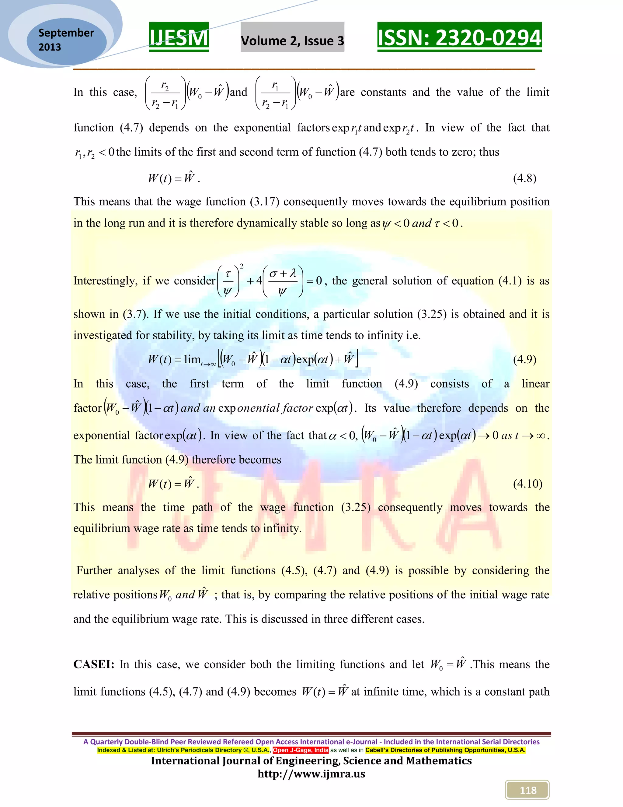
IJESM Volume 2, Issue 3 ISSN: 2320-0294 _________________________________________________________ A Quarterly Double-Blind Peer Reviewed Refereed Open Access International e-Journal - Included in the International Serial Directories Indexed & Listed at: Ulrich's Periodicals Directory ©, U.S.A., Open J-Gage, India as well as in Cabell’s Directories of Publishing Opportunities, U.S.A. International Journal of Engineering, Science and Mathematics http://www.ijmra.us 118 September 2013 In this case,  WW rr r ˆ 0 12 2        and  WW rr r ˆ 0 12 1        are constants and the value of the limit function (4.7) depends on the exponential factors tr1exp and tr2exp . In view of the fact that 0, 21 rr the limits of the first and second term of function (4.7) both tends to zero; thus WtW ˆ)(  . (4.8) This means that the wage function (3.17) consequently moves towards the equilibrium position in the long run and it is therefore dynamically stable so long as 00   and . Interestingly, if we consider 04 2                  , the general solution of equation (4.1) is as shown in (3.7). If we use the initial conditions, a particular solution (3.25) is obtained and it is investigated for stability, by taking its limit as time tends to infinity i.e.      WttWWtW t ˆexp1ˆlim)( 0    (4.9) In this case, the first term of the limit function (4.9) consists of a linear factor     tfactoronentialanandtWW  expexp1ˆ 0  . Its value therefore depends on the exponential factor  texp . In view of the fact that ,0       tasttWW 0exp1ˆ 0  . The limit function (4.9) therefore becomes WtW ˆ)(  . (4.10) This means the time path of the wage function (3.25) consequently moves towards the equilibrium wage rate as time tends to infinity. Further analyses of the limit functions (4.5), (4.7) and (4.9) is possible by considering the relative positions WandW ˆ 0 ; that is, by comparing the relative positions of the initial wage rate and the equilibrium wage rate. This is discussed in three different cases. CASEI: In this case, we consider both the limiting functions and let WW ˆ 0  .This means the limit functions (4.5), (4.7) and (4.9) becomes WtW ˆ)(  at infinite time, which is a constant path
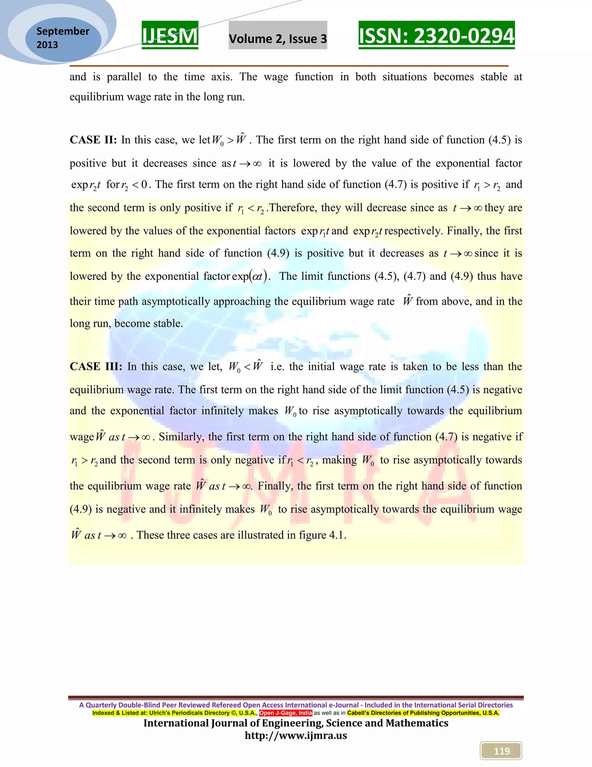
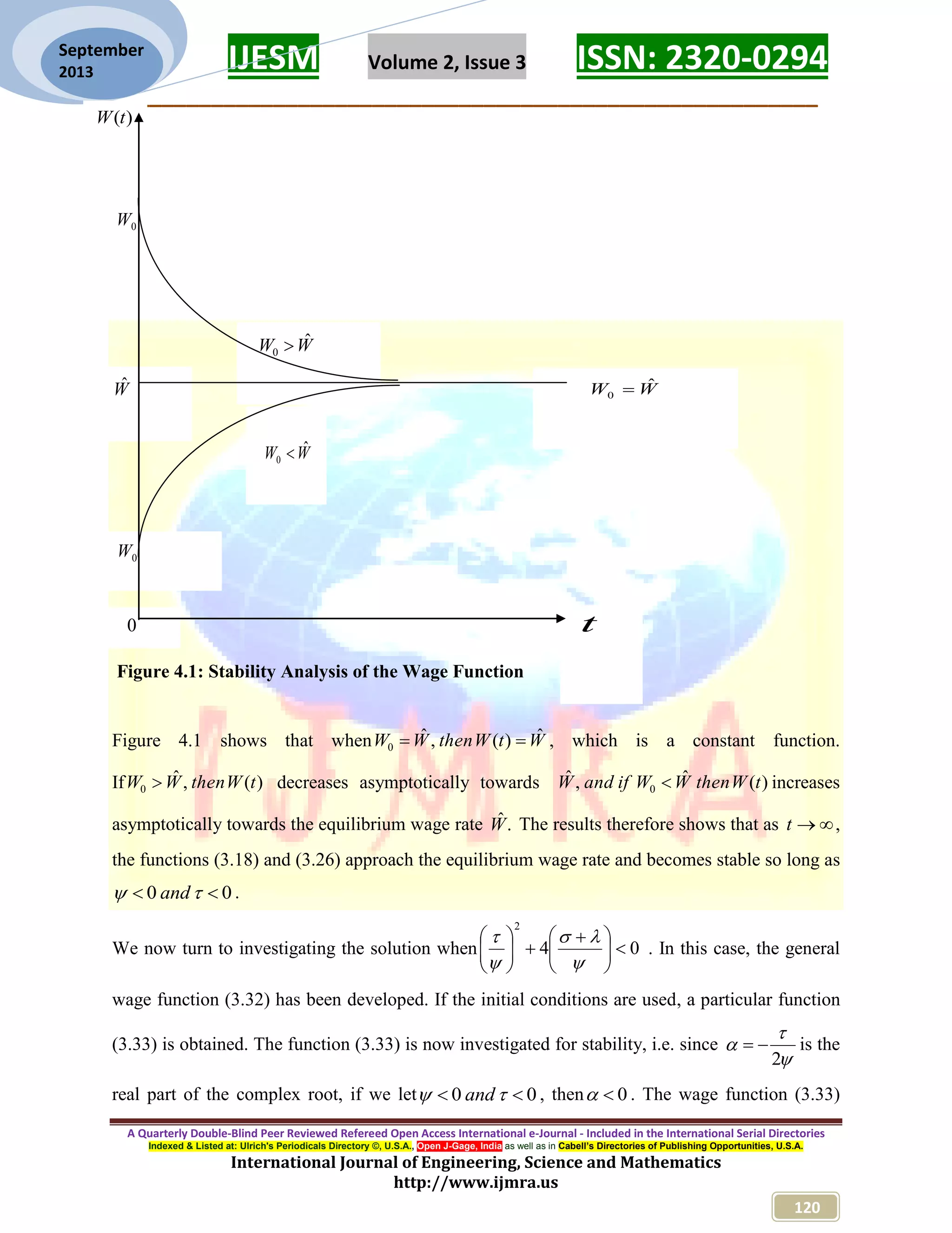
IJESM Volume 2, Issue 3 ISSN: 2320-0294 _________________________________________________________ A Quarterly Double-Blind Peer Reviewed Refereed Open Access International e-Journal - Included in the International Serial Directories Indexed & Listed at: Ulrich's Periodicals Directory ©, U.S.A., Open J-Gage, India as well as in Cabell’s Directories of Publishing Opportunities, U.S.A. International Journal of Engineering, Science and Mathematics http://www.ijmra.us 119 September 2013 and is parallel to the time axis. The wage function in both situations becomes stable at equilibrium wage rate in the long run. CASE II: In this case, we let WW ˆ 0  . The first term on the right hand side of function (4.5) is positive but it decreases since as t it is lowered by the value of the exponential factor tr2exp for 02 r . The first term on the right hand side of function (4.7) is positive if 21 rr  and the second term is only positive if 21 rr  .Therefore, they will decrease since as t they are lowered by the values of the exponential factors tr1exp and tr2exp respectively. Finally, the first term on the right hand side of function (4.9) is positive but it decreases as t since it is lowered by the exponential factor  texp . The limit functions (4.5), (4.7) and (4.9) thus have their time path asymptotically approaching the equilibrium wage rate Wˆ from above, and in the long run, become stable. CASE III: In this case, we let, WW ˆ 0  i.e. the initial wage rate is taken to be less than the equilibrium wage rate. The first term on the right hand side of the limit function (4.5) is negative and the exponential factor infinitely makes 0W to rise asymptotically towards the equilibrium wage tasWˆ . Similarly, the first term on the right hand side of function (4.7) is negative if 21 rr  and the second term is only negative if 21 rr  , making 0W to rise asymptotically towards the equilibrium wage rate .ˆ tasW Finally, the first term on the right hand side of function (4.9) is negative and it infinitely makes 0W to rise asymptotically towards the equilibrium wage tasWˆ . These three cases are illustrated in figure 4.1.
IJESM Volume 2, Issue 3 ISSN: 2320-0294 _________________________________________________________ A Quarterly Double-Blind Peer Reviewed Refereed Open Access International e-Journal - Included in the International Serial Directories Indexed & Listed at: Ulrich's Periodicals Directory ©, U.S.A., Open J-Gage, India as well as in Cabell’s Directories of Publishing Opportunities, U.S.A. International Journal of Engineering, Science and Mathematics http://www.ijmra.us 120 September 2013 Figure 4.1: Stability Analysis of the Wage Function Figure 4.1 shows that when WtWthenWW ˆ)(,ˆ 0  , which is a constant function. If )(,ˆ 0 tWthenWW  decreases asymptotically towards )(ˆ,ˆ 0 tWthenWWifandW  increases asymptotically towards the equilibrium wage rate .ˆW The results therefore shows that as t , the functions (3.18) and (3.26) approach the equilibrium wage rate and becomes stable so long as 00   and . We now turn to investigating the solution when 04 2                  . In this case, the general wage function (3.32) has been developed. If the initial conditions are used, a particular function (3.33) is obtained. The function (3.33) is now investigated for stability, i.e. since    2  is the real part of the complex root, if we let 00   and , then 0 . The wage function (3.33) )(tW 0W WW ˆ 0  Wˆ WW ˆ 0  0W WW ˆ 0  0 t
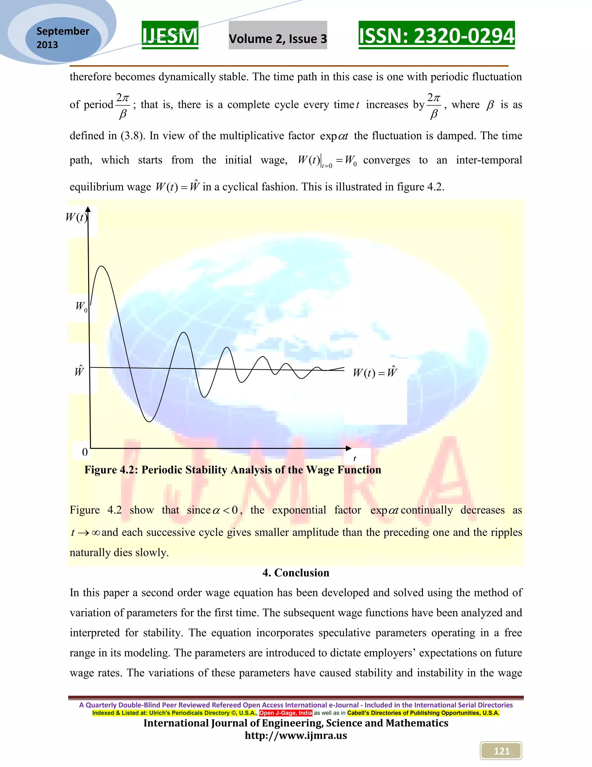
IJESM Volume 2, Issue 3 ISSN: 2320-0294 _________________________________________________________ A Quarterly Double-Blind Peer Reviewed Refereed Open Access International e-Journal - Included in the International Serial Directories Indexed & Listed at: Ulrich's Periodicals Directory ©, U.S.A., Open J-Gage, India as well as in Cabell’s Directories of Publishing Opportunities, U.S.A. International Journal of Engineering, Science and Mathematics http://www.ijmra.us 121 September 2013 therefore becomes dynamically stable. The time path in this case is one with periodic fluctuation of period  2 ; that is, there is a complete cycle every timet increases by  2 , where  is as defined in (3.8). In view of the multiplicative factor texp the fluctuation is damped. The time path, which starts from the initial wage, 00 )( WtW t  converges to an inter-temporal equilibrium wage WtW ˆ)(  in a cyclical fashion. This is illustrated in figure 4.2. Figure 4.2: Periodic Stability Analysis of the Wage Function Figure 4.2 show that since 0 , the exponential factor texp continually decreases as t and each successive cycle gives smaller amplitude than the preceding one and the ripples naturally dies slowly. 4. Conclusion In this paper a second order wage equation has been developed and solved using the method of variation of parameters for the first time. The subsequent wage functions have been analyzed and interpreted for stability. The equation incorporates speculative parameters operating in a free range in its modeling. The parameters are introduced to dictate employers’ expectations on future wage rates. The variations of these parameters have caused stability and instability in the wage )(tW 0W Wˆ WtW ˆ)(  0 t
IJESM Volume 2, Issue 3 ISSN: 2320-0294 _________________________________________________________ A Quarterly Double-Blind Peer Reviewed Refereed Open Access International e-Journal - Included in the International Serial Directories Indexed & Listed at: Ulrich's Periodicals Directory ©, U.S.A., Open J-Gage, India as well as in Cabell’s Directories of Publishing Opportunities, U.S.A. International Journal of Engineering, Science and Mathematics http://www.ijmra.us 122 September 2013 function in certain circumstances. Above all, where the wage function takes an exponential form with particular assumptions, as time approaches infinity it asymptotically approaches the equilibrium wage rate. Where as in a case of an exponential and a periodic factor, the time path shows a periodic function whose successive cycles elicit smaller amplitudes and the ripples eventually dies naturally at equilibrium wage rate as time approaches infinity. It has been realized that where the wage rate is determined by free market forces of demand and supply, volatility in wage rate may be observed if not controlled. This may increase uncertainties and cause anxiety about investment and employment in the economy. The paper therefore proposes government intervention by creating a middle path in which wage rate is allowed to oscillate freely within a narrow band managed by employers in consultation with the workers under the watch of the government. References 1. Alpha, C. Fundamental Methods of Mathematical Economics. Auckland: McGraw-Hill International Book Company, 1984, pp. 470-534. 2. Burton, T D. Introduction to Dynamic Systems Analysis. New York: McGraw-Hill, Inc, 1994, pp. 128-141. 3. Erwin, K. Advanced Engineering Mathematics. New York: John Wiley and Sons, Inc., 1993, pp. 1-126. 4. Glenn, L. Differential Equations: A modeling Approach. New York: McGraw-Hill Companies Inc., 2005, pp. 80-81. 5. Hostetler, R P and Larson, R E. Differential Equations to Accompany Calculus. Lexington: D.C. Heath and Company, 1980, pp. 46-57. 6. Oxforddictionaries.com/definition/english/wage, retrieved on Thursday 6th June, 2013. 7. Silas, N. O. etal, On the Walrasian-Samuelson Price Adjustment Model, Sofia: International Journal of Pure and Applied Mathematics, Volume 61, No. 2, 2010, 211-218. 8. Stroud, K. A. Advanced Engineering Mathematics. New York: Palgrave Macmillan, 2003, pp. 47-91. 9. www.thefreedictionary.com/wage, retrieved on Thursday 6th June, 2013. 10. www.vizualhr.com/hrguide/article:asp?article=88, retrieved on Thursday 6th June, 2013.

APPLICATION OF THE METHOD OF VARIATION OF PARAMETERS: MATHEMATICAL MODEL FOR DEVELOPING AND ANALYZING STABILITY OF THE WAGE FUNCTION

  • 1.
    IJESM Volume 2,Issue 3 ISSN: 2320-0294 _________________________________________________________ A Quarterly Double-Blind Peer Reviewed Refereed Open Access International e-Journal - Included in the International Serial Directories Indexed & Listed at: Ulrich's Periodicals Directory ©, U.S.A., Open J-Gage, India as well as in Cabell’s Directories of Publishing Opportunities, U.S.A. International Journal of Engineering, Science and Mathematics http://www.ijmra.us 107 September 2013 APPLICATION OF THE METHOD OF VARIATION OF PARAMETERS: MATHEMATICAL MODEL FOR DEVELOPING AND ANALYZING STABILITY OF THE WAGE FUNCTION Olala, Gilbert Owuor Abstract In this paper, a second order wage equation is developed and solved by the method of variation of parameters. The subsequent wage function is then analyzed and interpreted for stability. Speculative parameters, which operate freely dictating employers’ expectations, are included in modeling this equation. The variation of these parameters causes both stability and instability of the wage function depending on circumstances. Where the wage function is exponential, asymptotic stability towards the equilibrium wage rate is observed but where it consists of both exponential and periodic factors, the time path shows periodic fluctuations with successive cycles giving smaller amplitudes until the ripples die naturally. It has been realized that where the wage rate is determined by free market forces of demand and supply, volatility in wage rate may be observed if not controlled. This may increase uncertainties and cause anxiety about investment and employment in the economy. The paper therefore proposes government intervention by creating a middle path in which wage rate is allowed to oscillate freely within a narrow band managed by employers in consultation with the workers under the watch of the government. Key words: wage equation, wage function, wage rate, equilibrium wage rate, stability, market forces, volatile wage rate, and middle path.  Department of Mathematics & Computer Science, Kisumu Polytechnic, Kisumu, KENYA
  • 2.
    IJESM Volume 2,Issue 3 ISSN: 2320-0294 _________________________________________________________ A Quarterly Double-Blind Peer Reviewed Refereed Open Access International e-Journal - Included in the International Serial Directories Indexed & Listed at: Ulrich's Periodicals Directory ©, U.S.A., Open J-Gage, India as well as in Cabell’s Directories of Publishing Opportunities, U.S.A. International Journal of Engineering, Science and Mathematics http://www.ijmra.us 108 September 2013 1. Introduction Wages mean the reward for labor services. In [6] wage is defined as a fixed regular payment earned for work or services, typically paid on a daily or weekly basis. In [9] wage is viewed as payment for labour services to a worker, especially remuneration on an hourly, daily, weekly or by piece. It also views wage as a portion of national product that represents aggregate paid for all contributing labour and services as distinguished from the portion retained by management or reinvested in capital goods. In [10] wage is defined according to wages act of 1986. It is the sum payable to an employee by an employer in connection with that employment. It includes fees, bonuses, commissions, holiday pay or other emolument relevant to the employment whether specified in the contract of employment or not. In this paper, we consider modeling a second order differential wage equation. For example, considering deterministic price adjustment model in [7] fixed supply and demand functions at instantaneous price for security is discussed. It is argued that at equilibrium asset price, quantity demanded equals quantity supplied. This is discussed using fixed demand and supply curves while price is kept constant. It also asserts that away from the equilibrium, excess demand for security raises its price, and excess supply lowers its price. In this situation, it is argued that the sign for rate of change of price with respect to time depends on the sign of excess demand. If the demand and supply functions are made linear at constant equilibrium price, deterministic model of price adjustment is realized with respective sensitivities. In the analysis of the solution of the deterministic model, it was observed that in the long run asset price settles at a constant steady state where no further change can occur. In [4] a natural decay equation is developed. The equation describes a phenomenon where a quantity gradually decreases to zero. In the work, it is emphasized that convergence depends the sign of the proportionality parameter. If the proportionality parameter is negative then it turns into a growth equation but if it is positive, it stabilizes in the long run. In the study of slope fields for autonomous equations qualitative properties of decay equation is demonstrated. It was found that the solution could be positive, negative or zero. In all the three cases, the solution approaches zero in limit as time approaches infinity.
  • 3.
    IJESM Volume 2,Issue 3 ISSN: 2320-0294 _________________________________________________________ A Quarterly Double-Blind Peer Reviewed Refereed Open Access International e-Journal - Included in the International Serial Directories Indexed & Listed at: Ulrich's Periodicals Directory ©, U.S.A., Open J-Gage, India as well as in Cabell’s Directories of Publishing Opportunities, U.S.A. International Journal of Engineering, Science and Mathematics http://www.ijmra.us 109 September 2013 In [1], dynamics of market prices are studied. It was found out that if the initial price function lies off the equilibrium point, in the long run stability will be realized at the equilibrium position. It also brings out clear case by case analysis of the solution of second order price equation by introducing unrestricted parameters that brings speculations in behavior of buyers and sellers. The author argued that depending on the signs of these parameters, buyers will cut or increase their purchases. Similarly, sellers will cut or increase their supplies. It was also noted that depending on signs of parameters, price function stabilizes in the long run. In [2], equilibrium solutions about a special class of static solutions are discussed. The study found that if a system starts exactly at equilibrium position, then it remains there forever. The study further found that in real systems, small disturbances often a rise which moves a system away from equilibrium state. Such disturbances, regardless of their origin give rise to initial conditions which do not coincide with equilibrium condition. If the system is not at equilibrium point, then some of its derivatives will be non zero and the system therefore exhibits a dynamic behavior, which can be monitored by watching orbits in its phase space. The resistance-inductance electric current circuit for constant electromotive force is modeled into a differential equation in [3].The stability of the solution is studied in the long run and is found to be a constant, which is the ratio of constant electromotive force to resistance. It was also found that if electromotive force is periodic, in the long run, current executes harmonic oscillations. In this case, steady state solution is the periodic part of the solution. The resistance-capacitor electric current circuit equation is also discussed for constant electromotive force. The solution was an exponential function, which converges to zero in the long run. Also, in resistance- inductance-capacitance series circuit, a second order equation was developed. Its solution consists of an exponential homogeneous part and a periodic integral part. The study found out that the homogeneous part converges to zero as time approaches infinity, while the periodic part exhibits practically harmonic oscillations. The literature is silent and it is worthwhile developing a second order wage equation, solve it and discuss its stability. The solutions of linear second order ordinary differential equations are presented in [5; 8] using the method of variation of parameters.
  • 4.
    IJESM Volume 2,Issue 3 ISSN: 2320-0294 _________________________________________________________ A Quarterly Double-Blind Peer Reviewed Refereed Open Access International e-Journal - Included in the International Serial Directories Indexed & Listed at: Ulrich's Periodicals Directory ©, U.S.A., Open J-Gage, India as well as in Cabell’s Directories of Publishing Opportunities, U.S.A. International Journal of Engineering, Science and Mathematics http://www.ijmra.us 110 September 2013 2. Modeling second order wage equation In this section, we consider modeling a second order linear differential wage equation. In this case, the number demanded and supplied of labor is taken as functions both current wage rate and wage trend prevailing in the market at that time. This is because wage trend will guide laborers expectations regarding future wage level. The expectations will also influence labor demand and supply for future decision making. To include wage trend and expectations, we include continuous time derivatives in the model, i.e. dt dW (2.1) and 2 2 dt Wd (2.2) The derivative (2.1) shows whether the wage function is rising, and the derivative (2.2) shows whether it is rising at an increasing rate. If we consider wage trends, derivatives as additional arguments to labor demand and supply are taken into account. The demand and supply functions are thus given as        2 2 ,),( dt Wd dt dW tWfNd (2.3) and        2 2 ,),( dt Wd dt dW tWfNs (2.4) respectively. Suppose the demand and supply functions of labor are linear, then they are  0,,2 2   dt Wd dt dW WNd (2.5) and  0,,2 2   dt Wd dt dW WNs (2.6) respectively. The other parameters  and,, introduced to dictate employers and laborers expectations have their signs operating in free range. For example, if 0 , a rising wage rate causes the number of laborers demanded to increase. This suggest that employers expect rising wage rate to continue to rise and prefer to increase employment now when the
  • 5.
    IJESM Volume 2,Issue 3 ISSN: 2320-0294 _________________________________________________________ A Quarterly Double-Blind Peer Reviewed Refereed Open Access International e-Journal - Included in the International Serial Directories Indexed & Listed at: Ulrich's Periodicals Directory ©, U.S.A., Open J-Gage, India as well as in Cabell’s Directories of Publishing Opportunities, U.S.A. International Journal of Engineering, Science and Mathematics http://www.ijmra.us 111 September 2013 wage rate is still relatively low. On the other hand, for 0 , the wage trend will be falling, and employers will opt to cut current employment while waiting for wage rate to fall even further. The inclusion of the parameter  makes employers behavior to depend also on the rate of change of wage rate dt dW . Thus introducing new parameters  and injects wage rate speculation in the model. Similarly, if we let 0 , then a rising wage rate causes the number of laborers supplied to fall and thus laborers expect the rising wage rate to continue rising and prefer to withhold their services now while waiting for the higher wage rate. On the other hand, for 0 , wage rate will shows a falling trend and laborers will prefer to offer their services now while the wage rate is still relatively high hoping that any delay will see the wage rate fall even further. Therefore, introduction of the parameter  makes the behavior of laborers to depend much on the wage rate just as the employers. We now resort to demonstrating an implicit model by assuming that only labor demand function contains the wage expectations. Specifically, we set both  and of function (2.6) equal to zero; while  and of function (2.5) are set as non zero. Further, we assume that labor market clears at every point in time. We then set the number of laborers demanded equal to the number of laborers supplied to obtain equation bWa dt dW a dt Wd  212 2 (2.7) with                      bandaa ,, 21 , and this is the required second order linear ordinary differential wage equation. 3. Solution of the differential equation In this section, we demonstrate the solution of the differential equation (2.7) using the method of variation of parameters. We first solve equation (2.7) for a complementary solution by considering its homogeneous equation 0212 2  Wa dt dW a dt Wd . (3.1) The characteristic equation of equation (3.1) is
  • 6.
    IJESM Volume 2,Issue 3 ISSN: 2320-0294 _________________________________________________________ A Quarterly Double-Blind Peer Reviewed Refereed Open Access International e-Journal - Included in the International Serial Directories Indexed & Listed at: Ulrich's Periodicals Directory ©, U.S.A., Open J-Gage, India as well as in Cabell’s Directories of Publishing Opportunities, U.S.A. International Journal of Engineering, Science and Mathematics http://www.ijmra.us 112 September 2013 021 2  arar . (3.2) Equation (3.2) is quadratic in nature and can be solved for r using the quadratic formula. The roots are therefore given as 2 4 , 2 2 11 21 aaa rr   . (3.3) If we substitute back the values of 21 aanda as given in equation (2.7) the roots become                             4 2 1 , 2 21 rr . (3.4) The roots (3.4) yields varied results depending on the value of the discriminant                  4 2 . This is discussed in three cases. Case I: Suppose 04 2                  then roots 21 randr of the characteristic equation (3.2) are real and different. The complementary solution therefore becomes trctrctWc 2211 expexp)(  (3.5) Case II: Suppose 04 2                  then the roots 21 randr of the characteristic equation (3.2) are real and equal; that is,    2 , 21 rr (3.6) and the complementary solution then becomes   ttcctWc exp)( 21  . (3.7) Case III: Suppose 04 2                  then the roots 21 randr of the characteristic equation (3.2) are complex; that is,  irr 21, ,    2 with and                    4 2 1 2 (3.8) and the complementary solution therefore becomes
  • 7.
    IJESM Volume 2,Issue 3 ISSN: 2320-0294 _________________________________________________________ A Quarterly Double-Blind Peer Reviewed Refereed Open Access International e-Journal - Included in the International Serial Directories Indexed & Listed at: Ulrich's Periodicals Directory ©, U.S.A., Open J-Gage, India as well as in Cabell’s Directories of Publishing Opportunities, U.S.A. International Journal of Engineering, Science and Mathematics http://www.ijmra.us 113 September 2013  tctcttWc  sincosexp)( 21  (3.9) To solve equation (2.7) completely requires finding an integral function )(tWI by the method of variation of parameters. This is also discussed in three cases. Case I: Suppose 04 2                  the roots 21 randr are real and different, from the complementary solution (3.5), the integral function takes the form trvtrvtWI 2211 expexp)(  (3.10) toffunctionsarevandvwhere 21 . The system of equations to be solved is      btrrvtrrv trvtrv 222111 2211 expexp 0expexp (3.11) The system of equations is solved by Cramer’s rule for 21 vandv to obtain   21112 121 1 ,0,exp rrrtr rrr b v         (3.12) and   0,,exp 22122 221 2         rrrtr rrr b v (3.13) Substituting solutions (3.12) and (3.13) in integral solution (3.10) gives 0,,)( 21 21  rr rr b tWI (3.14) From solution (3.4), we have           21rr ; and since           b , the integral solution (3.14) becomes        ,ˆ)( WtWI (3.15) If we consider complementary solution (3.5) and integral solution (3.15), the general solution becomes WtrctrctW ˆexpexp)( 2211  (3.16)
  • 8.
    IJESM Volume 2,Issue 3 ISSN: 2320-0294 _________________________________________________________ A Quarterly Double-Blind Peer Reviewed Refereed Open Access International e-Journal - Included in the International Serial Directories Indexed & Listed at: Ulrich's Periodicals Directory ©, U.S.A., Open J-Gage, India as well as in Cabell’s Directories of Publishing Opportunities, U.S.A. International Journal of Engineering, Science and Mathematics http://www.ijmra.us 114 September 2013 The general solution (3.16) is solved for a particular solution if we use the initial conditions. Suppose 0)( 0 00    t t dt dW andWtW then the particular solution becomes     WtrWW rr r trWW rr r tW ˆexpˆexpˆ)( 20 12 1 10 12 2      (3.17) Case II: Suppose 04 2                  the roots 21 randr of the characteristic equation are real and equal. From solution (3.7), the integral function takes the form    ttvtvtWI  expexp)( 21  (3.18) where 21 vandv are functions oft . The system of equations to be solved is therefore                  bttvtv ttvtv   exp1exp 0expexp 21 21 (3.19) This is easily solved by Cramer’s rule for 21 vandv to obtain  tt bb v          exp21 (3.20) and  t b v    exp2 (3.21) The integral function is found by substituting solutions (3.20) and (3.21) in solution (3.18) to obtain 2 )(  b tWI  (3.22) But since 04 2                  ,                   2 2 2 and because           b from equation (2.7), the integral function becomes        ,ˆ)( WtWI (3.23) The general wage function is therefore found to be     WttcctW ˆexp)( 21   (3.24)
  • 9.
    IJESM Volume 2,Issue 3 ISSN: 2320-0294 _________________________________________________________ A Quarterly Double-Blind Peer Reviewed Refereed Open Access International e-Journal - Included in the International Serial Directories Indexed & Listed at: Ulrich's Periodicals Directory ©, U.S.A., Open J-Gage, India as well as in Cabell’s Directories of Publishing Opportunities, U.S.A. International Journal of Engineering, Science and Mathematics http://www.ijmra.us 115 September 2013 If we use initial conditions 0)( 0 00    t t dt dW andWtW then the particular solution becomes      WttWWtW ˆexp1ˆ)( 0   (3.25) Case III: Suppose 04 2                  the roots 21 randr of the characteristic equation (3.2) are complex. The roots (3.8) and the complementary solution (3.9), gives an integral function tivtivtWI )exp()exp()( 21   (3.26) where 21 vandv are functions oft . We use Cramer’s rule to solve for 21 vandv in the system                    )(expexp )(0expexp 21 21 bbtiivtiiv ativtiv   (3.27) to obtain    ti i b v )(exp 2 1      (3.28) and    ti i b v )(exp 2 2      (3.29) Substituting solutions (3.28) and (3.29) in the integral function (3.26) gives .)( 22    b tWI (3.30) But from solution (3.8),            22 and since           b the integral function (3.30) becomes .,ˆ)(       WtWI (3.31) The most general solution is thus written as   .ˆsincosexp)( 21 WtctcttW   (3.32) Solution (3.32) is solved for a particular solution if we use the initial conditions. Suppose we let 0)( 0 00    t t dt dW andWtW the particular solution becomes
  • 10.
    IJESM Volume 2,Issue 3 ISSN: 2320-0294 _________________________________________________________ A Quarterly Double-Blind Peer Reviewed Refereed Open Access International e-Journal - Included in the International Serial Directories Indexed & Listed at: Ulrich's Periodicals Directory ©, U.S.A., Open J-Gage, India as well as in Cabell’s Directories of Publishing Opportunities, U.S.A. International Journal of Engineering, Science and Mathematics http://www.ijmra.us 116 September 2013   WtWWtWWttW ˆsin)ˆ(cos)ˆ(exp)( 00            (3.33) 4. Results, analysis and interpretation In this paper, a second order wage equation bWa dt dW a dt Wd  212 2 (4.1) with                      bandaa ,, 21 has been developed for the first time. In this equation, 0 is a parameter that shows the number of laborers supplied that does not depend on the wage rate, 0 is a parameter that shows the proportion by which the number of laborers supplied responds to variation in wage rate, 0 a parameter that shows the number of laborers demanded that does not depend on wage rate, and 0 a parameter that shows the proportion by which the number of laborers demanded responds to variation in wage rate. The parameters  and introduced to dictate employers’ expectations have their signs operating in a free range. For example, if 0 , a rising wage rate causes number of laborers demanded to increase. This suggests that employer expects a rising wage rate to continue to rise and prefer to increase employment now when the wage rate is still relatively low. On the other hand for 0 , the wage rate shows a falling trend and employer will opt to cut employment now while waiting wage rate to fall even further. The parameter  makes the employer’s behavior to depend on the rate of change of wage rate. Equation (4.1) has been solved in this paper by the method of variation of parameters for the first time. When 04 2                  , the general solution was found as WtrctrctW ˆexpexp)( 2211  (4.2) with 21 randr described in solution (3.4), and Wˆ in solution (3.15). In this case, suppose 04,0            then and      ofvalues             ,04 2 . The solution (4.2) is
  • 11.
    IJESM Volume 2,Issue 3 ISSN: 2320-0294 _________________________________________________________ A Quarterly Double-Blind Peer Reviewed Refereed Open Access International e-Journal - Included in the International Serial Directories Indexed & Listed at: Ulrich's Periodicals Directory ©, U.S.A., Open J-Gage, India as well as in Cabell’s Directories of Publishing Opportunities, U.S.A. International Journal of Engineering, Science and Mathematics http://www.ijmra.us 117 September 2013 therefore valid. Moreover, with 0,sin,0   ce ,                  4 2 is positive and its square root exceeds . 2         Therefore solutions (3.4) produce one positive root 1r and one negative root 2r . Consequently, inter temporal equilibrium is dynamically unstable. For the function (4.2) to be stable, we have to set constant 1c to zero so that it becomes WtrctW ˆexp)( 22  (4.3) If we use the initial conditions 0)( 0 00    t t dt dW andWtW then solution (4.3) becomes   WtrWWtW ˆexpˆ)( 20  (4.4) The solution (4.4) is now investigated for stability by taking the limit as t tends to infinity, i.e.   WtrWWtW t ˆexpˆlim)( 20   (4.5) In this case,  WW ˆ 0  is constant and the value of limit function (4.5) depends on the exponential factor tr2exp . In view of the fact that ,02 r    tastrWW 0expˆ 20 . The limit function (4.5) therefore becomes WtW ˆ)(  . (4.6) This means time path of the wage function (4.4) consequently moves towards equilibrium position in the long run. Considering particular solution (3.17), suppose we let 0,0   with , the expression under the square root in solution (3.4) is less than 2         and the square root must be less than   ; therefore for ,0,04 2                   letweif then the roots of (3.4) would produce two negative roots. The solution (3.17) is therefore investigated for stability by finding its path, i.e.     WtrWW rr r trWW rr r tW ttt ˆlimexpˆlimexpˆlim)( 20 12 1 10 12 2                 . (4.7)
  • 12.
    IJESM Volume 2,Issue 3 ISSN: 2320-0294 _________________________________________________________ A Quarterly Double-Blind Peer Reviewed Refereed Open Access International e-Journal - Included in the International Serial Directories Indexed & Listed at: Ulrich's Periodicals Directory ©, U.S.A., Open J-Gage, India as well as in Cabell’s Directories of Publishing Opportunities, U.S.A. International Journal of Engineering, Science and Mathematics http://www.ijmra.us 118 September 2013 In this case,  WW rr r ˆ 0 12 2        and  WW rr r ˆ 0 12 1        are constants and the value of the limit function (4.7) depends on the exponential factors tr1exp and tr2exp . In view of the fact that 0, 21 rr the limits of the first and second term of function (4.7) both tends to zero; thus WtW ˆ)(  . (4.8) This means that the wage function (3.17) consequently moves towards the equilibrium position in the long run and it is therefore dynamically stable so long as 00   and . Interestingly, if we consider 04 2                  , the general solution of equation (4.1) is as shown in (3.7). If we use the initial conditions, a particular solution (3.25) is obtained and it is investigated for stability, by taking its limit as time tends to infinity i.e.      WttWWtW t ˆexp1ˆlim)( 0    (4.9) In this case, the first term of the limit function (4.9) consists of a linear factor     tfactoronentialanandtWW  expexp1ˆ 0  . Its value therefore depends on the exponential factor  texp . In view of the fact that ,0       tasttWW 0exp1ˆ 0  . The limit function (4.9) therefore becomes WtW ˆ)(  . (4.10) This means the time path of the wage function (3.25) consequently moves towards the equilibrium wage rate as time tends to infinity. Further analyses of the limit functions (4.5), (4.7) and (4.9) is possible by considering the relative positions WandW ˆ 0 ; that is, by comparing the relative positions of the initial wage rate and the equilibrium wage rate. This is discussed in three different cases. CASEI: In this case, we consider both the limiting functions and let WW ˆ 0  .This means the limit functions (4.5), (4.7) and (4.9) becomes WtW ˆ)(  at infinite time, which is a constant path
  • 13.
    IJESM Volume 2,Issue 3 ISSN: 2320-0294 _________________________________________________________ A Quarterly Double-Blind Peer Reviewed Refereed Open Access International e-Journal - Included in the International Serial Directories Indexed & Listed at: Ulrich's Periodicals Directory ©, U.S.A., Open J-Gage, India as well as in Cabell’s Directories of Publishing Opportunities, U.S.A. International Journal of Engineering, Science and Mathematics http://www.ijmra.us 119 September 2013 and is parallel to the time axis. The wage function in both situations becomes stable at equilibrium wage rate in the long run. CASE II: In this case, we let WW ˆ 0  . The first term on the right hand side of function (4.5) is positive but it decreases since as t it is lowered by the value of the exponential factor tr2exp for 02 r . The first term on the right hand side of function (4.7) is positive if 21 rr  and the second term is only positive if 21 rr  .Therefore, they will decrease since as t they are lowered by the values of the exponential factors tr1exp and tr2exp respectively. Finally, the first term on the right hand side of function (4.9) is positive but it decreases as t since it is lowered by the exponential factor  texp . The limit functions (4.5), (4.7) and (4.9) thus have their time path asymptotically approaching the equilibrium wage rate Wˆ from above, and in the long run, become stable. CASE III: In this case, we let, WW ˆ 0  i.e. the initial wage rate is taken to be less than the equilibrium wage rate. The first term on the right hand side of the limit function (4.5) is negative and the exponential factor infinitely makes 0W to rise asymptotically towards the equilibrium wage tasWˆ . Similarly, the first term on the right hand side of function (4.7) is negative if 21 rr  and the second term is only negative if 21 rr  , making 0W to rise asymptotically towards the equilibrium wage rate .ˆ tasW Finally, the first term on the right hand side of function (4.9) is negative and it infinitely makes 0W to rise asymptotically towards the equilibrium wage tasWˆ . These three cases are illustrated in figure 4.1.
  • 14.
    IJESM Volume 2,Issue 3 ISSN: 2320-0294 _________________________________________________________ A Quarterly Double-Blind Peer Reviewed Refereed Open Access International e-Journal - Included in the International Serial Directories Indexed & Listed at: Ulrich's Periodicals Directory ©, U.S.A., Open J-Gage, India as well as in Cabell’s Directories of Publishing Opportunities, U.S.A. International Journal of Engineering, Science and Mathematics http://www.ijmra.us 120 September 2013 Figure 4.1: Stability Analysis of the Wage Function Figure 4.1 shows that when WtWthenWW ˆ)(,ˆ 0  , which is a constant function. If )(,ˆ 0 tWthenWW  decreases asymptotically towards )(ˆ,ˆ 0 tWthenWWifandW  increases asymptotically towards the equilibrium wage rate .ˆW The results therefore shows that as t , the functions (3.18) and (3.26) approach the equilibrium wage rate and becomes stable so long as 00   and . We now turn to investigating the solution when 04 2                  . In this case, the general wage function (3.32) has been developed. If the initial conditions are used, a particular function (3.33) is obtained. The function (3.33) is now investigated for stability, i.e. since    2  is the real part of the complex root, if we let 00   and , then 0 . The wage function (3.33) )(tW 0W WW ˆ 0  Wˆ WW ˆ 0  0W WW ˆ 0  0 t
  • 15.
    IJESM Volume 2,Issue 3 ISSN: 2320-0294 _________________________________________________________ A Quarterly Double-Blind Peer Reviewed Refereed Open Access International e-Journal - Included in the International Serial Directories Indexed & Listed at: Ulrich's Periodicals Directory ©, U.S.A., Open J-Gage, India as well as in Cabell’s Directories of Publishing Opportunities, U.S.A. International Journal of Engineering, Science and Mathematics http://www.ijmra.us 121 September 2013 therefore becomes dynamically stable. The time path in this case is one with periodic fluctuation of period  2 ; that is, there is a complete cycle every timet increases by  2 , where  is as defined in (3.8). In view of the multiplicative factor texp the fluctuation is damped. The time path, which starts from the initial wage, 00 )( WtW t  converges to an inter-temporal equilibrium wage WtW ˆ)(  in a cyclical fashion. This is illustrated in figure 4.2. Figure 4.2: Periodic Stability Analysis of the Wage Function Figure 4.2 show that since 0 , the exponential factor texp continually decreases as t and each successive cycle gives smaller amplitude than the preceding one and the ripples naturally dies slowly. 4. Conclusion In this paper a second order wage equation has been developed and solved using the method of variation of parameters for the first time. The subsequent wage functions have been analyzed and interpreted for stability. The equation incorporates speculative parameters operating in a free range in its modeling. The parameters are introduced to dictate employers’ expectations on future wage rates. The variations of these parameters have caused stability and instability in the wage )(tW 0W Wˆ WtW ˆ)(  0 t
  • 16.
    IJESM Volume 2,Issue 3 ISSN: 2320-0294 _________________________________________________________ A Quarterly Double-Blind Peer Reviewed Refereed Open Access International e-Journal - Included in the International Serial Directories Indexed & Listed at: Ulrich's Periodicals Directory ©, U.S.A., Open J-Gage, India as well as in Cabell’s Directories of Publishing Opportunities, U.S.A. International Journal of Engineering, Science and Mathematics http://www.ijmra.us 122 September 2013 function in certain circumstances. Above all, where the wage function takes an exponential form with particular assumptions, as time approaches infinity it asymptotically approaches the equilibrium wage rate. Where as in a case of an exponential and a periodic factor, the time path shows a periodic function whose successive cycles elicit smaller amplitudes and the ripples eventually dies naturally at equilibrium wage rate as time approaches infinity. It has been realized that where the wage rate is determined by free market forces of demand and supply, volatility in wage rate may be observed if not controlled. This may increase uncertainties and cause anxiety about investment and employment in the economy. The paper therefore proposes government intervention by creating a middle path in which wage rate is allowed to oscillate freely within a narrow band managed by employers in consultation with the workers under the watch of the government. References 1. Alpha, C. Fundamental Methods of Mathematical Economics. Auckland: McGraw-Hill International Book Company, 1984, pp. 470-534. 2. Burton, T D. Introduction to Dynamic Systems Analysis. New York: McGraw-Hill, Inc, 1994, pp. 128-141. 3. Erwin, K. Advanced Engineering Mathematics. New York: John Wiley and Sons, Inc., 1993, pp. 1-126. 4. Glenn, L. Differential Equations: A modeling Approach. New York: McGraw-Hill Companies Inc., 2005, pp. 80-81. 5. Hostetler, R P and Larson, R E. Differential Equations to Accompany Calculus. Lexington: D.C. Heath and Company, 1980, pp. 46-57. 6. Oxforddictionaries.com/definition/english/wage, retrieved on Thursday 6th June, 2013. 7. Silas, N. O. etal, On the Walrasian-Samuelson Price Adjustment Model, Sofia: International Journal of Pure and Applied Mathematics, Volume 61, No. 2, 2010, 211-218. 8. Stroud, K. A. Advanced Engineering Mathematics. New York: Palgrave Macmillan, 2003, pp. 47-91. 9. www.thefreedictionary.com/wage, retrieved on Thursday 6th June, 2013. 10. www.vizualhr.com/hrguide/article:asp?article=88, retrieved on Thursday 6th June, 2013.