This paper proposes a highly flexible, robust, and efficient constraint handling approach for the solution of the optimal power flow (OPF) problem and this solution lies in the ability to solve the power system problem and avoid the mathematical traps. Centralized control of the power system has become inevitable, in the interest of secure, reliable, and economic operation of the system. In this work, OPF is solved by considering the three distinct objectives, generation cost minimization, power loss minimization, and enhancement of voltage stability index. These three objectives are solved separately by considering the evolutionary-based monarch butterfly optimization (MBO) algorithm. This MBO algorithm is validated on the IEEE 30 bus network and the obtained results are compared with differential evolution, particle swarm optimization, genetic algorithm, and Jaya algorithm. The obtained results reveal that among the various optimization algorithms considered in this work, the MBO evolves as the best algorithm for all three case studies.
![International Journal of Informatics and Communication Technology (IJ-ICT) Vol. 13, No. 3, December 2024, pp. 519~526 ISSN: 2252-8776, DOI: 10.11591/ijict.v13i3.pp519-526 519 Journal homepage: http://ijict.iaescore.com Application of monarch butterfly optimization algorithm for solving optimal power flow Chan-Mook Jung1 , Sravanthi Pagidipala2 , Surender Reddy Salkuti3 1 Department of Railroad and Civil Engineering, Woosong University, Daejeon, Republic of Korea 2 Department of Electrical Engineering, National Institute of Technology Andhra Pradesh (NIT-AP), Tadepalligudem, India 3 Department of Railroad and Electrical Engineering, Woosong University, Daejeon, Republic of Korea Article Info ABSTRACT Article history: Received Feb 20, 2024 Revised Jun 22, 2024 Accepted Aug 12, 2024 This paper proposes a highly flexible, robust, and efficient constraint- handling approach for the solution of the optimal power flow (OPF) problem and this solution lies in the ability to solve the power system problem and avoid the mathematical traps. Centralized control of the power system has become inevitable, in the interest of secure, reliable, and economic operation of the system. In this work, OPF is solved by considering the three distinct objectives, generation cost minimization, power loss minimization, and enhancement of voltage stability index. These three objectives are solved separately by considering the evolutionary-based monarch butterfly optimization (MBO) algorithm. This MBO algorithm is validated on the IEEE 30 bus network and the obtained results are compared with differential evolution, particle swarm optimization, genetic algorithm, and Jaya algorithm. The obtained results reveal that among the various optimization algorithms considered in this work, the MBO evolves as the best algorithm for all three case studies. Keywords: Economic operation Generation cost Loss minimization Optimal power flow Voltage stability This is an open access article under the CC BY-SA license. Corresponding Author: Surender Reddy Salkuti Department of Railroad and Electrical Engineering, Woosong University Jayang-Dong, Dong-Gu, Daejeon, 34606, Republic of Korea Email: surender@wsu.ac.kr 1. INTRODUCTION Electrical power systems are highly complex and they are constantly growing in size to meet the ever-increasing demands of the customers. An efficient economic operation and planning of power systems have always played a very important role in the power industry [1], [2]. Optimal power flow (OPF) is an efficient scheduling method of power network that has the goal of reducing the total production cost of participating generator units while satisfying all the constraints for safe and reliable power to the consumers. OPF is required for a stable, reliable, and secure power system, which basically involves optimizing an objective function [3], [4]. The goal of OPF is to find the values of control variables that satisfy the economic and technical factors of an entire power system. OPF has several applications as it has a major impact on the transmission system and it is considered a basic tool for real-time pricing in the electricity markets. Generally, there are 3 types of problems in the power network, i.e., economic dispatch (ED), load flow, and OPF [5]-[6]. The solution of OPF starts by solving the load flow equation. The tools of power systems including the various studies are used in energy management systems (EMS), to manage the transmission network safely and economically. The OPF program developed should be highly flexible and very versatile for use in the operation of the power system. There are several desirable features when looking for an OPF program from a planning standpoint. Programs that are highly flexible and very versatile are the most useful. Minimization of loss received very](https://image.slidesharecdn.com/2120840ijict-251022055839-b530ceef/75/Application-of-monarch-butterfly-optimization-algorithm-for-solving-optimal-power-flow-1-2048.jpg)
![ ISSN: 2252-8776 Int J Inf & Commun Technol, Vol. 13, No. 3, December 2024: 519-526 520 little attention. Solution methods for load shedding have also been proposed. Contingency-security constraints have been integrated into OPF formulation. It was concluded that there is remarkable progress in network modeling, optimization models, and numerical techniques. The OPF algorithms that were commercially available satisfied the full set of non-linear models and set of constraints on variables. There are several methodologies developed in the literature for the solution of this OPF problem, including the conventional/traditional approaches such as Newton’s method [7], gradient method [8], linear programming [9], non-linear programming [10], and interior-point [11] method. The evolutionary-based algorithms (artificial intelligence (AI) methods) like genetic algorithm (GA) [12], particle swarm optimization (PSO) [13], enhanced GA (EGA) [14], differential evolution (DE) [15], bacterial foraging algorithm [16], teaching learning-based optimization (TLBO) [17], Jaya algorithm [18], gravitational search algorithm (GSA) [19], and glowworm swarm optimization (GSO) algorithm [20]. The solution of any OPF is not sensitive to the selected initial point for easy decision-making for the operator. The complexity of the OPF has to be minimized and it should be user-friendly. Like conventional algorithms, evolutionary-based algorithms don’t guarantee the absolute optimization solution, however, they provide a rational solution closer to the global optimal solution. Therefore, researchers are in search of finding new evolutionary algorithms for solving practical problems. These algorithms find their application in various power engineering problems such as power system planning, operation, and analysis. To name a few are generator expansion planning, optimal network feeder routing, capacitor placement, reactive power optimization, economic load dispatch, power loss minimization, contingency ranking for voltage stability, load management including demand response and load shedding, control of flexible AC transmission systems, power flow, OPFs, optimal allocation of FACTS, and load frequency control. In this work, the monarch butterfly optimization (MBO) algorithm is used for the solution of the OPF problem. 2. OPF: PROBLEM FORMULATION OPF problem is solved to obtain the system control variables when the power system economy and security are of concern. An OPF is one of the components of the EMS. OPF is considered a complex and non-linear optimization problem, and its main aim is to get the best solution by determining the optimized control variables. It has been identified that the quality and the speed at which the OPF solution is achieved are greatly influenced by the load flow technique used for the solution of equality constraints and the optimization technique used for modifying the control variables. In general, the OPF objectives are classified into single and multiple objectives. Here, OPF is solved by selecting 3 distinct objectives and they are formulated next. The main focus is to solve OPF by identifying the suitable control variables to achieve an optimum solution by satisfying the system control and operation constraints [21]. Here, the generator's active powers (𝑃𝐺𝑖) and voltage magnitudes (𝑉𝐺𝑖), settings of tap changing transformers (𝑇𝑖) and shunt capacitor banks (𝑄𝐶𝐵,𝑖) are selected as control variables, and they are expressed as (1), 𝑢𝑇 = [𝑃𝐺2, . . , 𝑃𝐺,𝑁𝐺 , 𝑉𝐺1, . . , 𝑉𝐺,𝑁𝐺 , 𝑇1, . . , 𝑇𝑁𝑇, 𝑄𝐶𝐵,1 , . . , 𝑄𝐶𝐵,𝑁𝐶𝐵 ] (1) state variables for OPF are slack bus power (𝑃𝑠𝑙𝑎𝑐𝑘), load bus voltages (𝑉𝐿𝑖), generator reactive powers (𝑄𝐺𝑖) and power flow in transmission lines (𝑆𝑙𝑖), and it is expressed as (2). 𝑥𝑇 = [𝑃𝑠𝑙𝑎𝑐𝑘, 𝑉𝐿𝑖, … , 𝑉𝐿,𝑁𝐿 , 𝑄𝐺1, … , 𝑄𝐺,𝑁𝐺 , 𝑆𝑙1, … , 𝑆𝑙,𝑁𝑙 ] (2) Here the power flow is performed by supplying the initial values of control variables from their range based on experience. One needs to check whether the given objective function is optimized or not. If not, it modifies the control variables using some conventional or evolutionary-based optimization technique and performs another power flow solution. This process is repeated until the objective function is optimized [22]. OPF solution is achieved after solving a large number of solutions of load flows in tune with a set of specified values of consumer demand. In this paper, OPF is solved by solving the three objectives and they are formulated next. 2.1. Objective 1: generation cost (GC) minimization Total cost of generation is the sum of fuel costs of each generating unit [23], [24], and mathematically, it is formulated as (3), minimize GC = ∑ 𝐺𝐶𝑖(𝑃𝐺𝑖) 𝑁𝐺 𝑖=1 (3)](https://image.slidesharecdn.com/2120840ijict-251022055839-b530ceef/75/Application-of-monarch-butterfly-optimization-algorithm-for-solving-optimal-power-flow-2-2048.jpg)
![Int J Inf & Commun Technol ISSN: 2252-8776 Application of monarch butterfly optimization algorithm for solving optimal power flow (Chan-Mook Jung) 521 where, 𝐺𝐶𝑖(𝑃𝐺𝑖) = 𝑎𝑖 + 𝑏𝑖𝑃𝐺𝑖 + 𝑐𝑖𝑃𝐺𝑖 2 (4) 𝑎𝑖, 𝑏𝑖 and 𝑐𝑖 are the coefficients of generation costs. 𝑁𝐺 is number of generators. 2.2. Objective 2: power loss minimization This minimization of losses in a power network (𝑃𝑙𝑜𝑠𝑠) is considered as objective, and the control variables are regulated to achieve this objective. In every power network, there is a significant amount of transmission losses that cannot be eliminated completely but can be minimized to achieve the economical and reliable goals of the power system [25]-[27]. This objective is non-linear, and it is formulated as (5), minimize 𝑃𝑙𝑜𝑠𝑠 = ∑ 𝐺𝑖𝑗[𝑣𝑖 2 + 𝑣𝑗 2 − 2𝑣𝑖𝑣𝑗𝑐𝑜𝑠(𝛿𝑖 − 𝛿𝑗)] 𝑁𝑇𝐿 𝑖,𝑗=1 (5) 2.3. Objective 3: enhancement of voltage stability index (L-Index) In this work, to monitor the voltage stability of the power network L-index is used. It is formulated as the minimization of squared L-indices [28], and it is expressed as (6), minimize L − index = ∑ 𝐿𝑗 2 𝑛 𝑗=𝑁𝐺+1 = ∑ |1 − ∑ 𝐹𝑖𝑗 𝑉𝑖 𝑉𝑗 𝑁𝐺 𝑖=1 | 2 𝑛 𝑗=𝑁𝐺+1 (6) where j = 𝑁𝐺 + 1,…,n. 𝐹𝑖𝑗 = −[𝑌𝐿𝐿]−1[𝑌𝐿𝐺] and it is obtained from the 𝑌𝐵𝑢𝑠 matrix by splitting it into generators and load buses. 2.4. Constraints The goal of equality constraints is to achieve the balance between power generation, losses, and power absorbed by the loads [29], [30]. These constraints are expressed as (7) and (8). 𝑃𝐺𝑖 − 𝑃𝐷𝑖 = 𝑉𝑖 ∑ 𝑉 𝑗(𝐺𝑖𝑗𝑐𝑜𝑠𝛿𝑖𝑗 + 𝐵𝑖𝑗𝑠𝑖𝑛𝛿𝑖𝑗) 𝑛 𝑗=1 (7) 𝑄𝐺𝑖 − 𝑄𝐷𝑖 = 𝑉𝑖 ∑ 𝑉 𝑗(𝐺𝑖𝑗𝑠𝑖𝑛𝛿𝑖𝑗 − 𝐵𝑖𝑗𝑐𝑜𝑠𝛿𝑖𝑗) 𝑛 𝑗=1 (8) The real and reactive power output from the generator is restricted by [31]. 𝑃𝐺𝑖 𝑚𝑖𝑛 ≤ 𝑃𝐺𝑖 ≤ 𝑃𝐺𝑖 𝑚𝑎𝑥 (9) 𝑄𝐺𝑖 𝑚𝑖𝑛 ≤ 𝑄𝐺𝑖 ≤ 𝑄𝐺𝑖 𝑚𝑎𝑥 (10) Bus voltages in the power network must be within the specified limits [32]. The voltage limits of generator and load buses are restricted by (11) and (12). 𝑉𝐺𝑖 𝑚𝑖𝑛 ≤ 𝑉𝐺𝑖 ≤ 𝑉𝐺𝑖 𝑚𝑎𝑥 𝑖 = 1,2, … , 𝑁𝐺 (11) 𝑉𝐿𝑖 𝑚𝑖𝑛 ≤ 𝑉𝐿𝑖 ≤ 𝑉𝐿𝑖 𝑚𝑎𝑥 𝑖 = 1,2, … , 𝑁𝐿 (12) the reactive power support from the shunt capacitor banks is limited by [33], 𝑄𝐶𝐵,𝑖 𝑚𝑖𝑛 ≤ 𝑄𝐶𝐵,𝑖 ≤ 𝑄𝐶𝐵,𝑖 𝑚𝑎𝑥 𝑖 = 1,2, … , 𝑁𝐶𝐵 (13) constraints on tap positions of transformers are limited by [34], 𝑇𝑖 𝑚𝑖𝑛 ≤ 𝑇𝑖 ≤ 𝑇𝑖 𝑚𝑎𝑥 𝑖 = 1,2, … , 𝑁𝑇 (14) the power flow in transmission lines is restricted by (15). −𝑆𝑖𝑗 𝑚𝑎𝑥 ≤ 𝑆𝑖𝑗 ≤ 𝑆𝑖𝑗 𝑚𝑎𝑥 (15)](https://image.slidesharecdn.com/2120840ijict-251022055839-b530ceef/75/Application-of-monarch-butterfly-optimization-algorithm-for-solving-optimal-power-flow-3-2048.jpg)
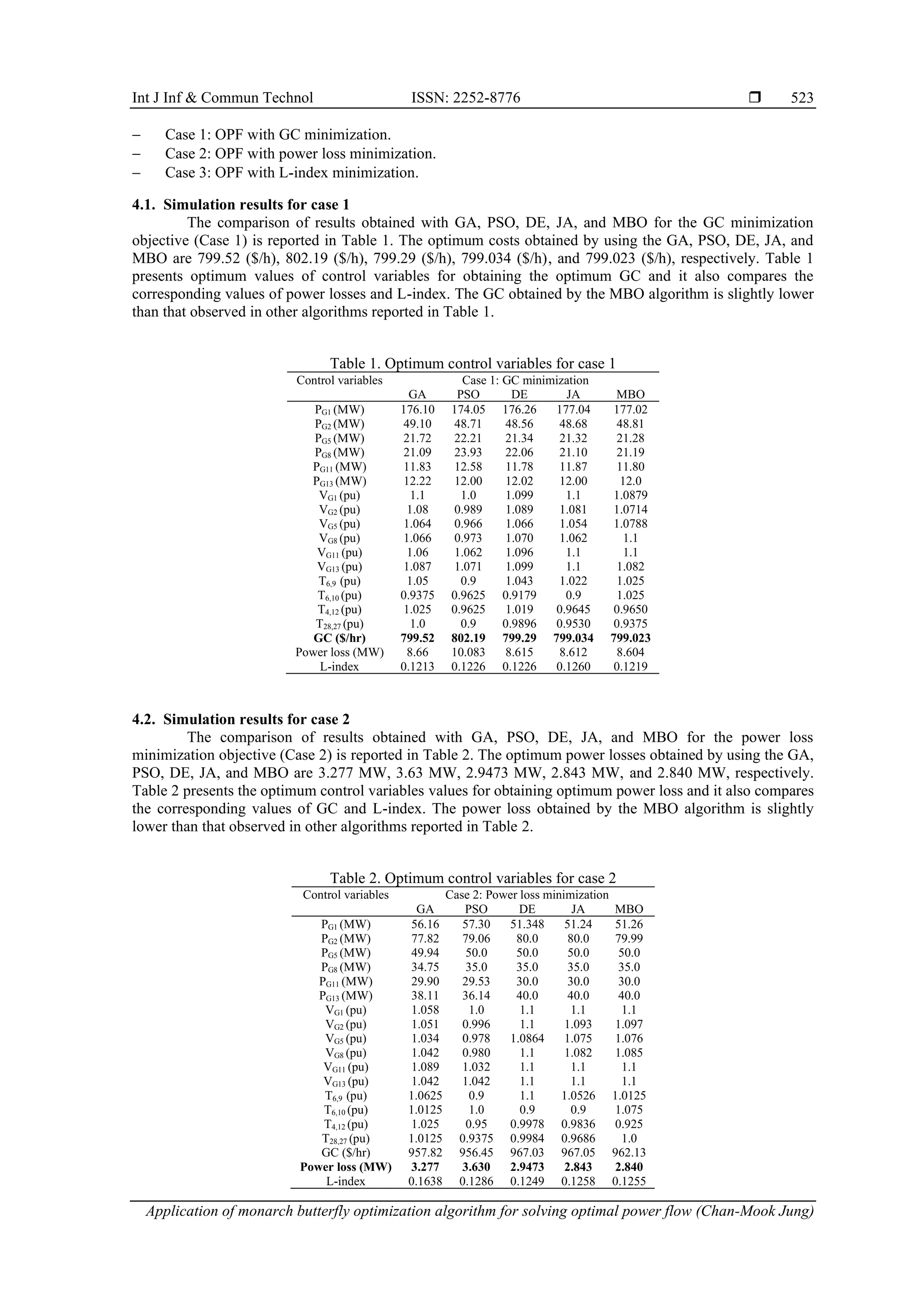
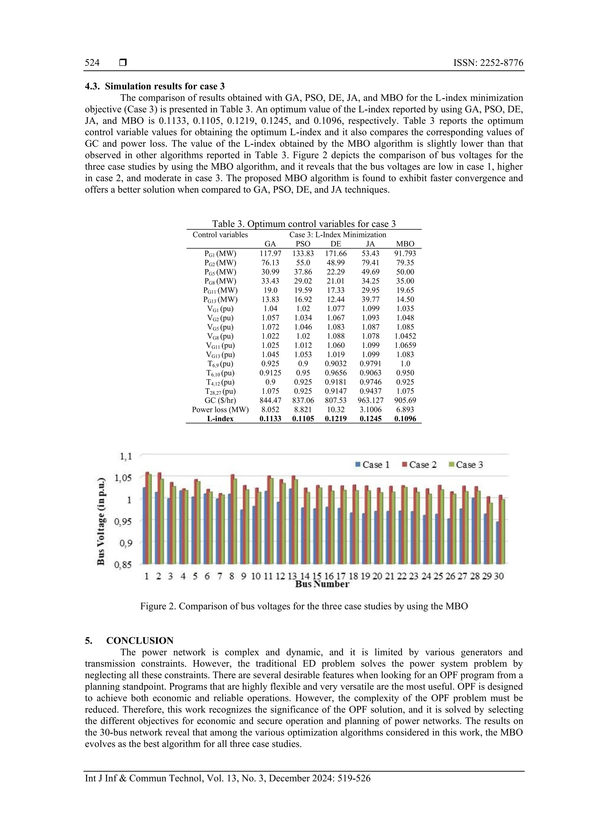
![ ISSN: 2252-8776 Int J Inf & Commun Technol, Vol. 13, No. 3, December 2024: 519-526 522 3. SOLUTION METHODOLOGY Before running an OPF, initially, a power flow program is executed to obtain a base case solution. One needs to determine the dependent and control variables for performing the OPF. In general, the solution of traditional OPF methods is affected by the initial guess of the solution. Also due to the non-linear nature of OPF, the solution of traditional OPF may fall in local optimum solution instead of reaching a global optimum solution. From a functional point of view, OPF combines the power flow problem and the ED problem. It is the best way to instantaneously operate the power system. MBO is an evolutionary-based technique that is developed based on the migration behavior of butterflies’ migration between two regions [35], [36]. During this migration, butterflies produce offspring and replace the corresponding parents. Mathematically, the entire process is divided into 2 updating operators namely the butterfly migration operator (BMO) and the butterfly adjustment operator (BAO). The detailed implementation details of MBO are reported in references [37]-[39]. The flowchart of solving the OPF using MBO is depicted in Figure 1. Figure 1. Flowchart of solving OPF using MBO 4. RESULTS AND DISCUSSION The effectiveness of the MBO algorithm is validated on the IEEE 30 bus system which has a total generation capacity of 900.2 MW. The complete details of this test system are taken from [40]. Selected tuned parameters of MBO for the OPF problem are: the period of migration is 1.2, the migration ratio is 5/12, the maximum step size is 1.0, and the butterfly adjusting rate is 5/12. In this paper, three cases are considered with different objectives, and they are: Read test system data, data related to MBO and maximum number of iterations Is iteration<max iteration? Yes No Increment iteration count Start Initialize all the parameters related to MBO, i.e., migration ratio, period of migration, adjustment rate and maximum step size Randomly generate the Monarch butterfly population Run power flow solution to determine the state vector Determine the violated constraints and assign fitness to each Monarch butterfly Compute the objective function and then determine the fitness function Sort the population based on the fitness of Monarch butterflies Divide the entire population of Monarch butterflies into two sub-populations Update the first subpopulation by using BMO Update the second subpopulation by using BAO Combined population (by merging two subpopulations) Determine the fitness function based on the objective to be optimized Store the optimum values of control variables and objective function under consideration STOP](https://image.slidesharecdn.com/2120840ijict-251022055839-b530ceef/75/Application-of-monarch-butterfly-optimization-algorithm-for-solving-optimal-power-flow-4-2048.jpg)
![Int J Inf & Commun Technol ISSN: 2252-8776 Application of monarch butterfly optimization algorithm for solving optimal power flow (Chan-Mook Jung) 525 ACKNOWLEDGEMENTS This research work was supported by “Woosong University’s Academic Research Funding - 2024”. REFERENCES [1] S. Frank and S. Rebennack, “An introduction to optimal power flow: Theory, formulation, and examples,” IIE Transactions, vol. 48, no. 12, pp. 1172-1197, 2016, doi: 10.1080/0740817X.2016.1189626. [2] B. Khan and P. Singh, “Optimal power flow techniques under characterization of conventional and renewable energy sources: a comprehensive analysis,” Journal of Engineering, vol. 2017, pp. 1-16, 2017, doi: 10.1155/2017/9539506. [3] S. Frank, I. Steponavice, and S. Rebennack, “Optimal power flow: a bibliographic survey I”, Energy Systems, vol. 3, pp. 221– 258, 2012, doi: 10.1007/s12667-012-0056-y. [4] B. Bentouati, S. Chettih, and L. Chaib, “Interior search algorithm for optimal power flow with non-smooth cost functions,” Cogent Engineering, vol. 4, no. 1, pp. 1-17, 2017, doi: 10.1080/23311916.2017.1292598. [5] A. Khan, H. Hizam, N. I. Abdul-Wahab, and M. L. Othman, “Solution of optimal power flow using non-dominated sorting multi objective based hybrid firefly and particle swarm optimization algorithm,” Energies, vol. 13, no. 16, 2020, doi: 10.3390/en13164265. [6] V. Yadav and S. P. Ghoshal, “Optimal power flow for IEEE 30 and 118-bus systems using monarch butterfly optimization,” Technologies for Smart-City Energy Security and Power, 2018, pp. 1-6, doi: 10.1109/ICSESP.2018.8376670. [7] B. V. Rao, G. V. N. Kumar, M. R. Priya, and P. V. S. Sobhan, “Optimal power flow by newton method for reduction of operating cost with SVC models,” International Conference on Advances in Computing, Control, and Telecommunication Technologies, 2009, pp. 468-470, doi: 10.1109/ACT.2009.121. [8] L. Gan and S. H. Low, “An online gradient algorithm for optimal power flow on radial networks,” IEEE Journal on Selected Areas in Communications, vol. 34, no. 3, pp. 625-638, Mar. 2016, doi: 10.1109/JSAC.2016.2525598. [9] P. Fortenbacher and T. Demiray, “Linear/quadratic programming-based optimal power flow using linear power flow and absolute loss approximations,” International Journal of Electrical Power and Energy Systems, vol. 107, pp. 680-689, 2019, doi: 10.1016/j.ijepes.2018.12.008. [10] S. Lee, H. Kim, and W. Kim, “Fast mixed-integer ac optimal power flow based on the outer approximation method,” Journal of Electrical Engineering and Technology, vol. 12, no. 6, pp. 2187-2195, 2017, doi: 10.5370/JEET.2017.12.6.2187. [11] Capitanescu, M. Glavic, D. Ernst, and L. Wehenkel, “Interior-point based algorithms for the solution of optimal power flow problems,” Electric Power Systems Research, vol. 77, no. 5–6, pp. 508-517, 2007, doi: 10.1016/j.epsr.2006.05.003. [12] T. M. Mohan and T. Nireekshana, “A genetic algorithm for solving optimal power flow problem,” 3rd International Conference on Electronics, Communication and Aerospace Technology, 2019, pp. 1438-1440, doi: 10.1109/ICECA.2019.8822090. [13] M. A. Abido, “Optimal power flow using particle swarm optimization,” International Journal of Electrical Power and Energy Systems, vol. 24, no. 7, pp. 563-571, 2002, doi: 10.1016/S0142-0615(01)00067-9. [14] A. G. Bakirtzis, P. N. Biskas, C. E. Zoumas, and V. Petridis, “Optimal power flow by enhanced genetic algorithm,” IEEE Transactions on Power Systems, vol. 17, no. 2, pp. 229-236, May 2002, doi: 10.1109/TPWRS.2002.1007886. [15] A. A. A. E. Ela, M. A. Abido, and S. R. Spea, “Optimal power flow using differential evolution algorithm,” Electric Power Systems Research, vol. 80, no. 7, pp. 878-885, 2010, doi: 10.1016/j.epsr.2009.12.018. [16] W. J. Tang, M. S. Li, Q. H. Wu, and J. R. Saunders, “Bacterial foraging algorithm for optimal power flow in dynamic environments,” IEEE Transactions on Circuits and Systems I: Regular Papers, vol. 55, no. 8, pp. 2433-2442, Sept. 2008, doi: 10.1109/TCSI.2008.918131. [17] H. R. E. H. Bouchekara, M. A. Abido, and M. Boucherma, “Optimal power flow using teaching-learning-based optimization technique,” Electric Power Systems Research, vol. 114, pp. 49-59, 2014, doi: 10.1016/j.epsr.2014.03.032. [18] W. Warid, H. Hizam, N. Mariun, and N. I. Abdul-Wahab, “Optimal power flow using the jaya algorithm,” Energies, vol. 9, no. 9, 2016, doi: 10.3390/en9090678. [19] S. R. Salkuti, “Feeder reconfiguration in unbalanced distribution system with wind and solar generation using ant lion optimization,” International Journal of Advanced Computer Science and Applications, vol. 12, no. 3, pp. 31-39, 2021, doi: 10.14569/IJACSA.2021.0120304. [20] S. Duman, U. Güvenç, Y. Sönmez, and N. Yörükeren, “Optimal power flow using gravitational search algorithm,” Energy Conversion and Management, vol. 59, pp. 86-95, 2012, doi: 10.1016/j.enconman.2012.02.024. [21] S. S. Reddy and C. S. Rathnam, “Optimal power flow using glowworm swarm optimization,” International Journal of Electrical Power and Energy Systems, vol. 80, pp. 128-139, 2016, doi: 10.1016/j.ijepes.2016.01.036. [22] S. R. Salkuti, “Multi-objective based optimal network reconfiguration using crow search algorithm,” International Journal of Advanced Computer Science and Applications, vol. 12, no. 3, pp. 86-95, 2021, doi: 10.14569/IJACSA.2021.0120310. [23] J. A. Arteaga, O. D. Montoya, and L. F. G. Noreña, “Solution of the optimal power flow problem in direct current grids applying the hurricane optimization algorithm,” Journal of Physics: Conference Series, vol. 1448, pp. 1-6, 2020, doi: 10.1088/1742- 6596/1448/1/012015. [24] S. R. Salkuti, “Optimal allocation of DG and D-STATCOM in a distribution system using evolutionary based bat algorithm,” International Journal of Advanced Computer Science and Applications, vol. 12, no. 4, pp. 360-365, 2021, doi: 10.14569/IJACSA.2021.0120445. [25] M. S. Kumari and S. Maheswarapu, “Enhanced genetic algorithm-based computation technique for multi-objective optimal power flow solution,” International Journal of Electrical Power and Energy Systems, vol. 32, no. 6, pp. 736-742, 2010, doi: 10.1016/j.ijepes.2010.01.010. [26] S. Karimullaand K. Ravi, “Solving multi objective power flow problem using enhanced sine cosine algorithm,” Ain Shams Engineering Journal, 2021, doi: 10.1016/j.asej.2021.02.037. [27] S. R. Salkuti, “Solving reactive power scheduling problem using multi-objective crow search algorithm,” International Journal of Advanced Computer Science and Applications, vol. 12, no. 6, pp. 42-48, 2021, doi: 10.14569/IJACSA.2021.0120606. [28] C. Coffrin, B. Knueven, J. Holzer, M. Vuffray, “The impacts of convex piecewise linear cost formulations on AC optimal power flow,” Electric Power Systems Research, vol. 199, 2021, doi: 10.1016/j.epsr.2021.107191. [29] X. Du, X. Lin, Z. Peng, S. Peng, J. Tang, W. Li, “Chance-constrained optimal power flow based on a linearized network model,” International Journal of Electrical Power & Energy Systems, vol. 130, 2021, doi: 10.1016/j.ijepes.2021.106890. [30] S. R. Salkuti, “Optimal operation of smart distribution networks using gravitational search algorithm,” International Journal of Advanced Computer Science and Applications, vol. 12, no. 6, pp. 531-538, 2021, doi: 10.14569/IJACSA.2021.0120661.](https://image.slidesharecdn.com/2120840ijict-251022055839-b530ceef/75/Application-of-monarch-butterfly-optimization-algorithm-for-solving-optimal-power-flow-7-2048.jpg)
![ ISSN: 2252-8776 Int J Inf & Commun Technol, Vol. 13, No. 3, December 2024: 519-526 526 [31] Y. Chen, J. Xiang, Y. Li, “A quadratic voltage model for optimal power flow of a class of meshed networks,” International Journal of Electrical Power & Energy Systems, vol. 131, 2021, doi: 10.1016/j.ijepes.2021.107047. [32] F. Zohrizadeh, C. Josz, M. Jin, R. Madani, J. Lavaei, S. Sojoudi, “A survey on conic relaxations of optimal power flow problem,” European Journal of Operational Research, vol. 287, no. 2, pp. 391-409, 2020, doi: 10.1016/j.ejor.2020.01.034. [33] J.S. Ferreira, E.J. de Oliveira, A.N. de Paula, L.W. de Oliveira, J.A.P. Filho, “Optimal power flow with security operation region,” International Journal of Electrical Power & Energy Systems, vol. 124, 2021, doi: 10.1016/j.ijepes.2020.106272. [34] W. Warid, “Optimal power flow using the AMTPG-Jaya algorithm,” Applied Soft Computing, vol. 91, 2020, doi: 10.1016/j.asoc.2020.106252. [35] P. Singh, N.K. Meena, J. Yang, E.V. Fuentes, S.K. Bishnoi, “Multi-criteria decision-making monarch butterfly optimization for optimal distributed energy resources mix in distribution networks”, Applied Energy, vol. 278, 2020, doi: 10.1016/j.apenergy.2020.115723. [36] Y. Feng, S. Deb, G.G. Wang, A.H. Alavi, “Monarch butterfly optimization: A comprehensive review,” Expert Systems with Applications, vol. 168, 2021, doi: 10.1016/j.eswa.2020.114418. [37] G. G. Wang, S. Deb, and Z. Cui, “Monarch butterfly optimization,” Neural Computing and Applications, vol. 31, pp. 1995–2014, 2019, doi: 10.1007/s00521-015-1923-y. [38] J. H. Yi, J. Wang, and G. G. Wang, “Using monarch butterfly optimization to solve the emergency vehicle routing problem with relief materials in sudden disasters,” Open Geosciences, vol. 11, no. 1, pp. 391-413, 2019, doi: 10.1515/geo-2019-0031. [39] Y. Feng, G. G. Wang, J. Dong, and L. Wang, “Opposition-based learning monarch butterfly optimization with Gaussian perturbation for large-scale 0-1 knapsack problem,” Computers and Electrical Engineering, vol. 67, pp. 454-468, 2018, doi: 10.1016/j.compeleceng.2017.12.014. [40] CASE_IEEE30 Power flow data for IEEE 30 bus test case, [Online]. Available.: https://matpower.org/docs/ref/matpower5.0/case_ieee30.html BIOGRAPHIES OF AUTHORS Chan-Mook Jung received Ph.D. Degree in railroad planning and bridge engineering from the Lehigh University, USA. Presently he is a professor at department of Railroad Civil System Engineering, Woosong University, Daejeon, Republic of Korea. His current research interests include railway demand forecasting, construction insurance, fatigue life evaluation, evaluation of railway ground stability, high-speed railways, railway tunnels, beam bridges analysis and optimization. He can be contacted at email: cmjung@wsu.ac.kr. Sravanthi Pagidipala is pursuing Ph.D. degree in electrical engineering at National Institute of Technology Andhra Pradesh (NIT-AP), Andhra Pradesh, India. Her research interests include renewable energy systems, microgrids, smart grids, energy conversion and management, energy and environmental economics, Ancillary Services Pricing, AI applications in electrical engineering, and multi-objective optimization. She can be contacted at email: pagidipala.nitap@gmail.com. Surender Reddy Salkuti received Ph.D. degree in electrical engineering from the Indian Institute of Technology (IIT), New Delhi, India, in 2013. He was a Postdoctoral Researcher at Howard University, Washington, DC, USA, from 2013 to 2014. He is currently an Associate Professor at the Department of Railroad and Electrical Engineering, Woosong University, Daejeon, Republic of Korea. His current research interests include market clearing, including renewable energy sources, demand response, and smart grid development with the integration of wind and solar photovoltaic energy sources. He can be contacted at email: surender@wsu.ac.kr.](https://image.slidesharecdn.com/2120840ijict-251022055839-b530ceef/75/Application-of-monarch-butterfly-optimization-algorithm-for-solving-optimal-power-flow-8-2048.jpg)