A petri net model for hardware software codesign

Design Automation for Embedded Systems, 4, 243–310 (1999) c 1999 Kluwer Academic Publishers, Boston. Manufactured in The Netherlands. A Petri Net Model for Hardware/Software Codesign PAULO MACIEL Departamento de Inform´ tica Universidade de Pernambuco CEP. 50732-970, Recife, Brazil a EDNA BARROS Departamento de Inform´ tica Universidade de Pernambuco CEP. 50732-970, Recife, Brazil a WOLFGANG ROSENSTIEL Fakultaet fuer Informatik Universitaet Tuebingen D-7207 Tuebingen, Germany Abstract. This work presents Petri nets as an intermediate model for hardware/software codesign. The main reason of using of Petri nets is to provide a model that allows for formal qualitative and quantitative analysis in order to perform hardware/software partitioning. Petri nets as an intermediate model allows one to analyze properties of the specification and formally compute performance indices which are used in the partitioning process. This paper highlights methods of computing load balance, mutual exclusion degree and communication cost of behavioral description in order to perform the initial allocation and the partitioning. This work is also devoted to describing a method for estimating hardware area, and it also presents an overview of the general partitioning method considering multiple software components. Keywords: Petri nets, hardware/software codesign, quantitative analysis, estimation 1. Introduction Because of the growing complexity of digital systems and the availability of technologies, nowadays many systems are mixed hardware/software systems. Hardware/software codesign is the design of systems composed of two kinds of components: application specific components (often referred to as hardware) and general programmable ones (often referred to as software). Although such systems have been designed ever since hardware and software first came into being, there is a lack of CAD tools to support the development of such heterogeneous systems. The progress obtained by the CAD tools at the level of algorithm synthesis, the advance in some key enabling technologies, the increasing diversity and complexity of applications employing embedded systems, and the need for decreasing the costs of designing and testing such systems all make techniques for supporting hardware/software codesign an important research topic [21, 22, 23, 24, 25]. The hardware/software codesign problem consists in implementing a given system func- tionally in a set of interconnected hardware and software components, taking into account design constraints. In the case where an implementation on a microprocessor (software component), cheap programmable component, does not meet the timing constraints [2], specific hardware devices must be implemented. On the other hand, to keep cost down, an implementation of components in software should be considered.

244 MACIEL, BARROS, AND ROSENSTIEL Furthermore, a short time-to-market is an important factor. The delay in product launching causes serious profit reductions, since it is much simpler to sell a product if you have little or no competition. It means that facilitating the re-use of previous designs, faster design exploration, qualitative analysis/verification in an early phase of the design, prototyping, and the reduction of the required time-to-test reduce the overall time required from a specification to the final product. One of the main tasks when implementing such systems is the partitioning of the description. Some partitioning approaches have been proposed by De Micheli [20], Ernst [18], Wolf [4] and Barros [17]. The hardware/software cosynthesis method developed by De Micheli et al. considers that the system-level functionality is specified with Hardware as a set of interacting processes. Vulcan-II partitions the system into portions to be implemented either as dedicated hardware modules or as a sequence of instructions on processors. This choice must be based on the feasibility of satisfaction of externally imposed data-rate constraints. The partitioning is carried out by analyzing the feasibility of partitions obtained by gradually moving hardware functions to software. A partition is considered feasible when it implements the original specification, satisfying performance indices and constraints. The algorithm is greedy and is not designed to find global minimums. Cosyma is a hardware/software codesign system for embedded controllers developed by Ernst et al. at University of Braunschweig. This system uses a superset of C language, called C∗ , where some constructors are used for specifying timing constraints and parallelism. The hardware/software partitioning in Cosyma is solved with simulated annealing. The cost function is based on estimation of hardware and software runtime, hardware/software communication time and on trace data. The main restriction of such a partitioning method is that hardware and software parts are not allowed for concurrent execution. The approach proposed by Wolf uses an object-oriented structure to partition functionality considering distributed CPUs. The specification is described at two levels of granularity. The system is represented by a network of objects which send messages among themselves to implement tasks. Each object is described as a collection of data variables and methods. The partitioning algorithm splits and recombines objects in order to speed up critical operations, although the splitting is only considered for the variable sets and does not explore the code sections. One of the challenges of hardware/software partitioning approaches is the analysis of a great varity of implementation alternatives. The approach proposed by Barros [14, 17, 16, 15] partitions a description into hardware and software components by using a clustering algorithm, which considers the distinct implementation alternatives. By considering a particular implementation alternative as the current one, clustering is carried out. The analysis of distinct implementation alternatives in the partitioning allows for the choice of a good implementation with respect to time constraints and area allocation. However, this method does not present a formal approach for performing quantitative analysis, and only considers a single processor architecture. Another very important aspect is the formal basis used in each phase of the design process. Layout models have a good formal foundation based on set and graph theory since this deals with placement and connectivity [94]. Logic synthesis is based on boolean algebra because

A PETRI NET MODEL 245 most of the algorithms deal with boolean transformation and minimization of expressions [95]. At high-level synthesis a lot of effort has been applied to this topic [96, 97, 98]. However, since high-level synthesis is associated to a number of different areas, varying from behavioral description to metric estimation, it does not have a formal theory of its own [9]. Software generation is based on programming languages which vary from logical to functional language paradigms. Since hardware/software codesign systems take into account a behavioral specification in order to provide a partitioned system as input for high- level synthesis tools and software compilers, they must consider design/implementation aspects of hardware and software paradigms. Therefore, a formal intermediate format able to handle behavioral specification that would also be relevant to hardware synthesis and software generation is an important challenge. Petri nets are a powerful family of formal description techniques able to model a large variety of problems. However, Petri nets are not only restricted to design modeling. Several methods have been developed for qualitative analysis of Petri net models. These methods [28, 29, 37, 26, 27, 30, 31, 1] allow for qualitative analysis of properties such as deadlock freedom, boundedness, safeness, liveness, reversibility and so on [42, 37, 87, 39]. This work extends Barros’s approach by considering the use of timed Petri nets as a formal intermediate format [61, 59] and takes into account a multi-processor architecture. In this work, the use of timed Petri nets as an intermediate format is mainly for computing metrics such as execution time, load balance [72], communication cost [70, 69], mutual exclusion degree [73] and area estimates [75]. These metrics guide the hardware/software partitioning. The next section is an introduction to the PISH codesign methodology. Section 3 introduces the description language adopted. Section 4 describes the hardware/software partitioning approach. Section 5 is an introduction to Petri nets [1, 64, 56, 58]. Section 6 presents the occam-time Petri net translation method [64, 59, 61, 62, 40]. Section 7 describes the approach adopted for performing qualitative analysis. A method for computing critical path time, minimal time and the likely time based on structural Petri net methods is presented in Section 8. Section 9 presents the extended model and an algorithm for estimating the number of processors needed. Section 10 describes the delay estimation method adopted in this work. Sections 11, 12, 13 and 14 describe methods for computing communication cost, load balance, mutual exclusion degree and area estimates, respectively. Section 15 presents an example and finally some conclusions and perspectives for future works follow. 2. The PISH Co-Design Methodology: An Overview The PISH co-design methodology being developed by a research group at Universidade de Pernambuco, uses occam as its specification language and comprises all phases of the design process, as depicted in Figure 1. The occam specification is partitioned into a set of processes, where some sets are implemented in software and others in hardware. The partitioning is carried out in such a way that the partitioned description is formally proved to have the same semantics as the original one. The partitioning task is guided by the metrics computed in the analysis phase. Processes for communication purposes are also generated

246 MACIEL, BARROS, AND ROSENSTIEL Figure 1. PISH design flow. in the partitioning phase. A more detailed description of the partitioning approach is given in Section 4. After partitioning, the processes to be implemented in hardware are synthesized and the software processes are compiled. The technique proposed for software compilation is also formally verified [93]. For hardware synthesis, a set of commercial tools has been used. First system prototype has been generated by using two distinct prototyping environments: The HARP board developed by Sundance and a transputer plus FPGAs boards, both connected through a PC bus. Once the system is validated, either the hardware components or the whole system can be implemented as an ASIC circuit. For this purpose, layout synthesis techniques for Sea-of-gates technology have been used [94]. 3. A Language for Specifying Communicating Processes The goal of this section is to present the language which is used both to describe the applications and to reason about the partitioning process itself. This language is a representative subset of occam, defined here by the BNF-style syntax definition showed below, where [clause] has the usual meaning of an optional item. The optional argument rep stands for a replicator. A detailed description of these constructors can be found in [62]. This subset of occam has been extended to consider two new constructors: BOX and CON. The syntax of these constructors is BOX P and CON P, where P is a process. These constructors have no semantic effect. They are just annotations, useful for the classification and the clustering phases. A process included within a BOX constructor is not split and its cost is analyzed as a whole at the clustering phase. The constructor CON is an annotation for a controlling process. Those processes act as an interface between the processes.

A PETRI NET MODEL 247 The occam subset is described in BNF format: P: : = SKIP STOP x: = e nop, deadlock and assignment ch?x ch!e input and output IF(c1 p1 , . . . , cn pn ) ALT(g1 p1 , . . . , gn pn ) conditional and non-deterministic conditional SEQ( p1 , . . . , pn ) PAR( p1 , . . . , pn ) sequential and parallel combiners WHILE(c P) while loop VAR x: P variable declaration CHAN ch: P channel declaration Occam obeys a set of algebraic laws [62] which defines its semantics. For example, the laws PAR( p1 , p2 ) = PAR( p2 , p1 ) and SEQ( p1 , p2 , . . . , pn ) = SEQ( p1 , SEQ( p2 , . . . , pn )) define the symmetry of the PAR constructor and the associativity of the SEQ constructor, respectively. 4. The Hardware/Software Partitioning Due to the computational complexity of optimum solution strategies, a need has arisen for a simplified, suboptimum approach to the partitioning system. In [20, 14, 18, 10, 11] some heuristic algorithms to the partitioning problem are presented. Recently, some works [12, 13] have suggested the use of formal methods for the partitioning process. However, although these approaches use formal methods to hardware/software partitioning, neither of them includes a formal verification that the partitioning preserves the semantics of the original description. The work reported in [16] presents some initial ideas towards a partitioning approach whose emphasis is correctness. This was the basis for the partitioning strategy presented here. As mentioned, the proposed approach uses occam [62] as a description language and suggests that the partitioning of an occam program should be performed by applying a series of algebraic transformations into the program. The main reason to use occam is that, being based on CSP [60], occam has a simple and a elegant semantics, given in terms of algebraic laws. In [63] the work is further developed, and a complete formalization of one of the partitioning phases, the splitting, is presented. The main idea of the partitioning strategy is to consider the hardware/software partitioning problem as a program transformation task, in all its phases. To accomplish this, an extended strategy to the work proposed in [16] has been developed, adding new algebraic transformation rules to deal with some more complex occam constructors such as replica- tors. Moreover, the proposed method is based on clustering and takes into account multiple software components. The partitioning method uses Petri nets as a common formalism [41] which allows for a quantitative analysis in order to perform the partitioning, as well as the qualitative analysis of the systems so that it is possible to detect errors in an early phase of the design [33].

248 MACIEL, BARROS, AND ROSENSTIEL Figure 2. Task diagram. 4.1. The Partitioning Approach: An Overview This section presents an overview of our proposed partitioning approach. The partitioning method is based on clustering techniques and formal transformations; and it is guided by the results of the quantitative analysis phase [61, 69, 70, 72, 73, 75]. The task-flow of the partitioning approach can be seen in Figure 2. This work extends the method presented in [15] by allowing to take into account a more generic target architecture. This must be defined by the designer by using the architecture generator, a graphical interface for specifying the number of software components, their interconnection as well as the memory organisation. The number and architecture of each hardware component will be defined during the partitioning phase. The first step in the partitioning approach is the splitting phase. The original description is transformed into a set of concurrent simple processes. This transformation is carried out by applying a set of formal rewriting rules which assures that the semantics is preserved [63]. Due to the concurrent nature of the process, communication must be introduced

A PETRI NET MODEL 249 among sequential data dependent processes. The split of the original description in simple processes allows a better exploration of the design space in order to find the best partitioning. In the classification phase, a set of implementation alternatives is generated. The set of implementation alternatives is represented by a set of class values concerning some features of the program, such as degree of parallelism and pipeline implementation. The choice of some implementation alternative as the current one can be made either manually or automatically. When choosing automatically, the alternatives lead to a balanced degree of parallelism among the various statements and the minimization of the area-delay cost function. Next, the occam/timed Petri net translation takes place. In this phase the split program is translated into a timed Petri net. In the qualitative analysis phase, a cooperative use of reduction rules, matrix algebra approach and reachability/coverability methods is applied to the Petri net model in order to analyze the properties of the description. This is an important aspect of the approach, because it allows for errors to be detected in an early phase of the design and, of course, decreases the design costs [33]. After that, the cost analysis takes place in order to find a partition of the set of processes, which fulfills the design constraints. In this work, the quantitative analysis is carried out by taking into account the timed Petri net representation of the design description, which is obtained by a occam/timed Petri net translation tool. Using a powerful and formal model such as Petri nets as intermediate format allows for the formal computation of metrics and for performing a more accurate cost estimation. Additionally, it makes the metrics computation independent of a particular specification language. In the quantitative analysis, a set of methods for performance, area, load balance and mutual exclusion estimation have been developed in the context of this work. The results of this analysis are used to reason about alternatives for implementing each process. After this, the initial allocation takes place. The term initial allocation is used to describe the initial assignment of one process to each processor. The criteria used to perform the initial allocation is the minimization of the inter-processor communication, balancing of the workload and the mutual exclusion degree among processes. One of the main problems in systems with multiple processors is the degradation in throughput caused by saturation effects [68, 66]. In distributed and multiple processor systems [65, 67], it is expected that doubling the number of processors would double the throughput of the system. However, experience has showed that throughput increases significantly only for the first few additional processors. Actually, at some point, throughput begins to decrease with each additional processor. This decrease is mainly caused by excessive inter-processor communication. The initial allocation method is based on a clustering algorithm. In the clustering phase, the processes are grouped in clusters considering one implementation alternative for each process. The result of the clustering process is an occam description representing the obtained clustering sequence with additional information indicating whether processes kept in the same cluster should be serialized or not. The serialization leads to the elimination of the unnecessary communication introduced during the splitting phase. A correct partitioned description is obtained after the joining phase, where transformation rules are applied again in order to combine processes kept in the same cluster and to eliminate

250 MACIEL, BARROS, AND ROSENSTIEL communication among sequential processes. In the following each phase of the partitioning process is explained with more detail. 4.2. The Splitting Strategy As mentioned, the partitioning verification involves the characterization of the partitioning process as a program transformation task. It comprises the formalization of the splitting and joining phases already mentioned. The goal of the splitting phase is to permit a flexible analysis of the possibilities for combining processes in the clustering phase. During the splitting phase, the original description is transformed into a set of simple processes, all of them in parallel. Since in occam PAR is a commutative operator, combining processes in parallel allows an analysis of all the permutations. The simple processes obey the normal form given below. chanch 1 , ch 2 , . . . , ch n : PAR(P1 , P2 , . . . , Pk ) where each Pi , 1 < i < k is a simple process. Definition 4.1 (Simple Process). A process P is defined as a simple if it is primitive (SKIP, STOP, x: = e, ch ? x, ch ! e), or has one of the following forms: (i.) ALT(b, &gk ck : = true) (ii.) IF(bk ck : = true) (iii.) BOX Q, HBOX Q and SBOX Q, where Q is an arbitrary process. (iv.) IF(c Q, TRUE SKIP) where Q is primitive or a process as in (i), (ii) or (iii). (v.), where Q is simple and are communication commands, possibly combined in sequence or in parallel. (vi.) WHILE c Q, where Q is simple. (vii.) VAR x: Q, where Q is simple. (viii.) CON Q, where Q is simple. This normal form expresses the granularity required by the clustering phase and this transformation permits a flexible analysis of the possibilities for combining processes in that phase. In [63] a complete formalization of the splitting phase can be found. To perform each one of the splitting and joining phases, a reduction strategy is necessary. The splitting strategy developed during the PISH project has two main steps. 1. the simplification IF and ALT processes 2. the parallelisation of the intermediary description generated by Step 1. The goal of Step 1 is to transform the original program into one in which all IFs and ALTs are simple processes. To accomplish this, occam laws have been applied. Two of these rules can be seen in Figure 3. The Rule 4.1.1 deals with conditionals. This rule transforms an arbitrary conditional into a sequence of IFs, with the aim to achieve the granularity required by the normal form. The application of this rule allows a flexible analysis of each sub-process of a conditional in the clustering phase. Note that the role of the first IF operator on the right-hand side of the rule above is to make the choice and to allow the subsequent conditionals to be carried out in sequence. This is why the fresh variables are necessary. Otherwise, execution of one conditional can interfere

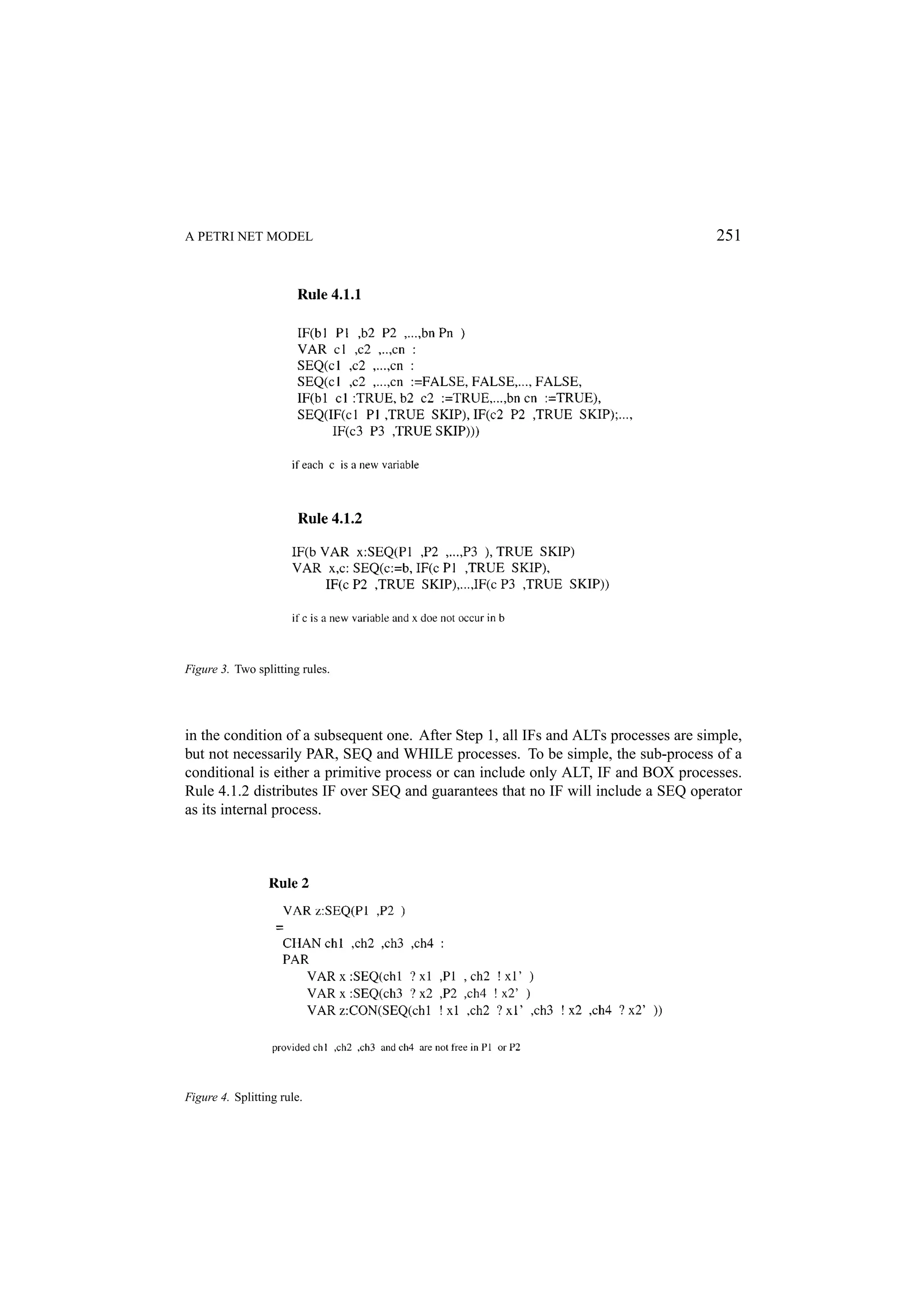
A PETRI NET MODEL 251 Figure 3. Two splitting rules. in the condition of a subsequent one. After Step 1, all IFs and ALTs processes are simple, but not necessarily PAR, SEQ and WHILE processes. To be simple, the sub-process of a conditional is either a primitive process or can include only ALT, IF and BOX processes. Rule 4.1.2 distributes IF over SEQ and guarantees that no IF will include a SEQ operator as its internal process. Figure 4. Splitting rule.

252 MACIEL, BARROS, AND ROSENSTIEL The goal of Step 2 is to transform the intermediate description generated by Step 1 into a simple form stated by the definition given above where all processes are kept in parallel. This can be carried out by using four additional rules. Rule 2 is an example of these rules, which puts in parallel two original sequential processes. In this rule, z is a list of local variables of S E Q(P1 , P2 ), x1 is a list of variables used and assigned in Pi and xi is a list of variables assigned in Pi . Assigned variables must be passed because one of Pi may have a conditional command including an assignment that may or not be executed. The process annotated with the operator CON is a controlling process, and this operator has no semantic effect. It is useful for the clustering phase. This process acts as an interface between the processes under its control and the rest of the program. Observe that the introduction of local variables and communication is essential, because processes can originally share variables (the occam language does not allow variable sharing between parallel processes). Obviously, there are other possible forms of introducing communication than that expressed in Rule 2. This strategy, however, allows for having control of the introduced communication, which makes the joining phase easier. Moreover, although it may seem expensive to introduce communication into the system, this is really necessary to allow a complete parallelisation of simple processes. The joining phase must be able to eliminate unnecessary communication between final processes. After the Step 2, the original program has been transformed into a program obeying the normal form. 4.3. The Partitioning Algorithm The technique for hardware/software process partitioning is based on the approach proposed by Barros [14, 15], which includes a classification phase followed by clustering of processes. These phases will be explained with more detail in this section. The considered version of such an approach did not cope with hierarchy in the initial specification, and only fixed size loops had been taken into account in the cost analysis. Additionally, the underlying architecture template considered only one software component (i.e. only one microprocessor or microcontroller), which limits the design space exploration. This work addresses some of these lacks by using Petri nets as an intermediate format, which support abstraction concepts and provide a framework for an accurate estimation of communication, area and delay cost, as well as load balance and mutual exclusion between processes. Additionally, the partitioning can taken into account more complexes architectures, which can be specified by the designer through a graphical environment. The occam/Petri net translation method and the techniques for a quantitative analysis will be later explained, respectively. 4.3.1. Classification In this phase a set of implementation possibilities represented as values of predefined attributes is attached to each process. The attributes were defined in order to capture the kind of communication performed by the process, the degree of parallelism inside the

A PETRI NET MODEL 253 Figure 5. Classiﬁcation and clustering phases. process (PAR and REPPAR constructors), whether the assignments in the process could be performed in pipeline (in the case of REPSEQ constructor) and the multiplicity of each process. As an example, Figure 5a illustrates some implementation alternatives for the process, which has a REPPAR constructor. Concerning distinct degrees of parallelism, all assignments inside this process can be implemented completely parallel, partially parallel or completely sequential. Although a set of implementation possibilities is attached to each process, only one is taken into account during the clustering phase and the choice can be done automatically or manually. In the case of an automatic choice, a balance of the parallelism degree of all implementations is the main goal. 4.3.2. The Clustering Algorithm Once a current alternative of implementation for each process has been chosen, the clustering process takes place. The ﬁrst step is the choice of some process to be implemented in the software components. This phase is called initial allocation [74] and may be controlled by the user or may be automatically guided by the minimization of a cost function. Taking into account the Petri net model, a set of metrics is computed and used for allocating

254 MACIEL, BARROS, AND ROSENSTIEL one process to each available software component. The allocation is a very critical task, since the partitioning of processes in software or hardware clusters depends on this initial allocation. The developed allocation method is also based on clustering techniques and groups processes in clusters by considering criteria such as communication cost [69, 70], functional similarity, mutual exclusion degree [73] and load balancing [72]. The number of resulting clusters is equal to the number of the software components in the architecture. From each cluster obtained, one process is chosen to be implemented in each software component. In order to implementing this strategy, techniques for calculating the degree of mutual exclusion between processes, the work load of processors, the communication cost and the functional similarity of processes have been defined and implemented. The partitioning of processes has been performed using a multi-stage hierarchical clustering algorithm [74, 15]. First a clustering tree is built as depicted in Figure 5.b. This is performed by considering criteria like similarity among processes, communication cost, mutual exclusion degree and resource sharing. In order to measure the similarity between processes, a metric has been defined, which allows for quantifying the similarity between two processes by analyzing the communication cost, the degree of parallelism of their current implementation, the possibility of implementing both processes in pipeline and the multiplicity of their assignments [15]. The cluster set is generated by cutting the clustering tree at the level (see Figure 5.b), which minimizes a cost function. This cost function considers the communication cost as well as area and delay estimations [75, 72, 61, 59, 15]. Below a basic clustering algorithm is described. First, a clustering tree is built based on a distance matrix. This matrix provides the distance between each two objects: p1 p2 p3 p4 0 d1 d2 d3 p1 0 d4 d5 p2 D = 0 d6 p3 0 p4 Algorithm 1. Begin with a disjoint clustering having level L(0) = 0 and sequence number m = 0. 2. Find the least dissimilar pair r , s of clusters in the current clustering according to d(r, s) = min{d(oi , o j )}. 3. Increment the sequence number (m ← m + 1). Merge the clusters r and s into a simple one in order to form the next clustering m. Set the level of this clustering to L(m) = d(r, s). 4. Update the distance matrix by deleting the row and the column corresponding to the clusters. The distance between the new cluster and an old cluster k may be defined as: d(k, (r, s)) = Max{d(k, r ), d(k, s)}, d(k, (r, s)) = Min{d(k, r ), d(k, s)} or d(k, (r, s)) = Average{d(k, r ), d(k, s)}. 5. Whether all objects are in one cluster, stop. Otherwise, go to the step 2.

A PETRI NET MODEL 255 After the construction of the clustering tree, this tree is cut by a cut-line. The cut-line makes clusters according to a cut-function. In order to allow the formal generation of a partitioned occam description in the joining phase, the clustering output is an occam description with annotations, which reflects the structure of the clustering tree, indicating whether resources should be shared or not. 4.4. The Joining Strategy Based on the result of the clustering and on the description obtained in the splitting, the joining phase generates a final description of the partitioned program in the form: chan: ch 1 , ch 2 , . . . , ch n : PAR(S1 , . . . , Ss , H1 , . . . , Hr ) where each Si and Hj are the generated clusters. Each of these is either one simple process (Pk ) of the split phase of a combination of some (Pk )’s. Also, none of the (Pk )’s is left out: each one is included in exactly one cluster. In this way, the precise mathematical notion of partition is captured. The Si , by convention, stands for the a software process and each Hj for a hardware process. Like the splitting phase, the joining phase should be designed as a set of transformation rules. Some of these rules are simply the inverses of the ones used in the splitting phase, but new rules for eliminating unnecessary communication between processes of a same cluster have been implemented [63]. The goal of the joining strategy is to eliminate irrelevant communication in the same cluster and after joining branches of conditionals and ALT processes as well as reducing sequences of parallel and sequential processes. The joining phase is inherently more difficult than splitting. The combination of simple processes results in a process which is not simple anymore. Therefore, no obvious normal form is obtained to characterize the result of the joining in general. Also, one must take a great care for not introducing deadlock when serializing processes in a given cluster. Also, in this phase some sequential processes are carried out in parallel, by applying some transformation rules. 5. A Brief Introduction to Petri Nets Petri nets are a powerful family of formal description techniques with a graphic and mathematical representation, and have powerful methods which allow for performing qualitative and quantitative analysis [37, 28, 29, 64]. This section presents a brief introduction to Place/Transitions nets and Timed Petri nets. 5.1. Place/Transition Nets Place/Transition Nets are bipartite graphs represented by two types of vertices called places (circles) and transitions (rectangles), interconnected by directed arcs (see Figure 6).

256 MACIEL, BARROS, AND ROSENSTIEL Figure 6. Simple Petri net. Place/Transition nets can be defined in terms of matrix as follow: Definition 5.1 (Place Transition Net). is defined as 5-tuple N = (P, T, I, O, M0 ), where P is a finite set of places which represents the state variables, T is a set of transitions which represents the set of actions, I : P × T → N is the input matrix which represents the pre-conditions, O: P × T → N is the output matrix which represents the post-conditions and M0 : P → N is the initial marking which represents the initial state. Definition 5.2 (Firing Rule). One transition t j is enabled to fire if, and only if, all its input places ( p ∈ P) has M( p) ≥ I ( p, t j ). The transition firing changes the marking of the net (M0 [t j > M ). The new marking is obtained as follows: M ( p) = M0 ( p) − I ( p, t j ) + O( p, t j ), ∀ p ∈ P The execution of actions is represented by the transition firing. However there are two particular cases where the firing rule is different: the first case is represented by source transitions. One source transition does not have any input places. This transition is always enabled. In the second case the transition does not have any output place. This transition is called of sink transition. Its firing does not create any token. Using the matrix representation, the structure of the net is represented by a set of places, a set of transitions, an input matrix (pre-conditions) and an output matrix (post-conditions). When one transition t fires, the difference between the markings is represented by O( p, t)− I ( p, t), ∀ p ∈ P. The matrix C = O − I is called incidence matrix. This matrix represents the structure of the net and if the net does not have self-loop. Definition 5.3 (Incidence Matrix). Let a net N = (P, T, I, O). The incidence matrix represents the relation C: P ×T → Z , ∀ p ∈ P defined by: C( p, t) = O( p, t)− I ( p, t), ∀ p ∈ P. A net that has self-loop may be represented by the incidence matrix if the self-loop is refined using dummy pair [37]. The state equation describes the behavior of the system, as well as allows for the analysis of properties of the models. Using matrix representation, the transition t j is represented by

A PETRI NET MODEL 257 a vector s, where the components of the vector are zero except for the j − th component, which is one. So it is possible to represent a marking either as M ( p) = M0 ( p) − I ( p, t j ) + O( p, t j ) or as M ( p) = M0 ( p) − I.s(t j ) + O.s(t j ) = M ( p) = M0 ( p) − C.s(t j )T , ∀ p ∈ P. Applying the sequence sq = t0 , . . . , tk , . . . , t0 , . . . , tn of transitions to the equation above, the following equation is obtained M ( p) = M0 ( p) + C.¯ , s where s = s(t0 )T , s(t1 )T , . . . , s(tn )T is called Parikh vector. ¯ The Place/Transition nets can be divided into several classes [28]. Each class has distinct modeling power. The use of subclasses improves the decision power of the models, although without excessively decreasing the modeling power. 5.2. Analysis The methods used to analyze Petri nets may be divided into three classes. The first method is graph-based and it builds on the reachability graph (reachability tree). The reachability graph is initial marking dependent and so it is used to analyse behavioral properties [39]. The main problem in the use of reachability tree is the high computational complexity [43, 44, 45, 46, 47, 48, 49, 50, 51, 52, 53, 54, 55] even if some interesting techniques are used such as: reduced graphs, graph symmetries, symbolic graph etc [35, 36]. The second method is based on the state equation [34, 37, 84, 86]. The main advantage of this method over the reachability graph is the existence of simple linear algebraic equations that aid in determining properties of the nets. Nevertheless, it gives only necessary or sufficient condition to the analysis of properties when it is applied to general Petri nets. The third method is based on reduction laws [37, 38]. The reduction laws based method provides a set of transformation rules which reduces the size of the models, preserving the properties. However, it is possible that for a given system and some set of rules, the reduction can not be complete. From a pragmatic point of view, it is fair to suggest that a better, more efficient and more comprehensive analysis can be done by a cooperative use of these techniques. Nevertheless, necessary and sufficient conditions can be obtained by applying the matrix algebra for some subclasses of Petri nets [33].

258 MACIEL, BARROS, AND ROSENSTIEL 5.3. Timed Petri Nets So far, Petri nets have been used to model a logical point of view of the systems; no formal attention has been given to temporal relations and constraints [71, 78, 76]. The first temporal approach was proposed by Ramchandani [57]. Today, there are at least three approaches which associate time to the nets: stochastic, firing times specified by intervals and deterministic. In the stochastic nets a probability distribution to the firing time is assigned to the model [80, 79]. Time can be associated with places (Place-Timed Models) [83], tokens (Token-Timed Models) [82] and transitions (Transition-Timed Petri Models). The approach proposed in [71] associates to each transition a time interval (dmin , dmax ) (Transition-Time Petri Nets). In deterministic timed nets the transitions firing can also be represented by policies: the first one is the three phase policy firing semantics and the second model is the atomic firing semantics approach. In the deterministic timed net with three phase policy semantics, the time information represents the duration of the transition’s firing [57]. The deterministic timed net with atomic firing may be represented by the approach proposed at [71] where time interval bounds are the same (di , di ) (Transition-Time Petri Nets). This section deals with the Timed Petri Nets, or rather, Petri net extensions in which the time information is expressed by duration (deterministic timed net with three phase policy firing semantics) and it is associated to the transitions. Definition 5.4 (Timed Petri Nets). Let a pair N t = (N , D) be a timed Petri net, where N = (P, T, I, O, M0 ) is a Petri net, D: T → R+ ∪ 0, is a vector which associates to each transition ti the duration of the firing di . A state in a Timed Petri Net is defined as 3-tuple of functions, one of which is the marking of the places; the second is the distribution in firing transitions and the last is the remaining firing time [77], for instance, if the number of tokens in a firing transition ti is mt (ti ) = k, then the remaining firing time is represented by a vector RT (t) = (r t (t)1 , . . . , r t (t)k ). More formally: Definition 5.5 (State of Timed Petri Net). Let N t = (N , D) a Timed Petri Net, a state S of N t is defined by a 3-tuple S = (M, M T, RT ), where M: P → N is the marking, M T : T → N is the distribution of tokens in the firing transitions and RT : K → R+ is the T remaining firing time function which assigns the remaining firing time to each independent firing of a transition for each transition that mt (t) = 0. K is the number of tokens in a firing transition ti (mt (ti ) = K ). RT is undefined for the transitions ti which mt (ti ) = 0. A transition ti obtaining concession at a time x is obliged to fire at the time, if there is no conflict. Definition 5.6 (Enabling Rule). Let N t = (N , D) be a Timed Petri Net, and S = (M, M T, RT ) the state of N t. We say that a bag of transitions BT is enabled at the instant

A PETRI NET MODEL 259 x if, and only if, M( p) ≥ ∀ti ∈BT #BT (ti ) × I ( p, ti ), ∀ p ∈ P, where BT (ti ) ⊆ BT and #BT (ti ) ∈ N. If a bag of transitions BT is enabled at the instant x, thus at that instant it removes from the input places of the bag BT the corresponding number of tokens (#BT (ti ) × I ( p, ti )) and, at the time x + di (di is the duration related to the transition ti in the bag BT ), adds the respective number of tokens in the output place. The number of tokens stored in the output place is equal to the product of the output arc weight (I ( p, t)) by the module of the bag regarding each transition t which has the duration equal to di (#BT (t), BT (t) ⊆ BT ) plus the number of tokens already “inside” the firing transitions, such that their duration have elapsed, during the present bag firing. Definition 5.7 (Firing Rule). Let N t = (N , D) be a Timed Petri Net, and S = (M, M T, RT ) the state of N t. If a bag of transitions BT is enabled at the instant x, then at the instant x ∀ti ∈BT #BT (ti ) × I ( p, ti ), ∀ p ∈ P number of tokens is removed from the input places of the bag BT . At the time x + d, the reached marking is M = M − ∀ti ∈BT #BT (ti )× I ( p, ti )+ ∀ti ∈BT |di =d #BT (ti )× O( p, ti )+ ∀tj ∈T,M T (tj )>0 M(t j ) × O( p, t j ), ∀ p ∈ P, if no other transition t ∈ T has been fired in the interval (x, x + di ). The inclusion of time in the Petri net models allows for performance analysis of systems. Section 8 introduces performance analysis in a Petri net context paying special attention to structural approaches of deterministic models. 6. The Occam—Petri Net Translation Method The development of a Petri net model of occam opens a wide range of applications based on qualitative analysis methods. To analyze performance aspects one requires a timed net model that represents the occam language. In our context, an occam program is a behavioral description which has to be implemented combining software and hardware components. Thus, the timing constraints applied to each operations of the description is already known, taking into account either hardware or software implementation. This section presents a timed Petri net model of occam language. This model allows for the execution time of the activities to be computed using the methods described in Sections 10 and 8. The occam-Petri net translation method [61] receives an occam description and translates it into a timed Petri net model. The occam programming language is derived from CSP [60], and allows the specification of parallel algorithms as a set of concurrent processes. An occam program is constructed by using primitive processes and process combiners as described in Section 3. The simplest occam processes are the assignment, the input action, the output action, the skip process and the stop process. Herewith, due to space restriction, only one primitive

260 MACIEL, BARROS, AND ROSENSTIEL Figure 7. Communication. process as well as one combiner will be described. A more detailed description can be found in [59, 61, 64]. 6.1. Primitive Communication Process: Input and Output Occam processes can send and receive messages synchronously through channels by using input (?) and output (!) operations. When a process receives a value through a channel, this value is assigned to a variable. Figure 7.b gives a net representing the input and the output primitive processes of the example in Figure 7.a. The synchronous communication is correctly represented by the net. It should be observed that the communication action is represented by the transition t0 and is only ﬁred when both the sender and the receiver processes are ready, which are represented by tokens in the places p0 and p1 . When a value is sent by an output primitive process through ch 1 , it is received and assigned to the variable x, being represented in the net by the data part of the model. Observe that the transition t1 can only be ﬁred when the places p2 and p3 have tokens. After that, both processes become enabled to execute the next actions.

A PETRI NET MODEL 261 Figure 8. Parallel. 6.2. Parallelism The combiner Par is one of the most powerful of the occam language. It permits concurrent process execution. The combined processes are executed simultaneously and only finish when every one has finished. Figure 8.a shows a program containing two processes t1 and t2 . Figure 8.b shows a net that represents the control of this program. One token in the place p0 enables the transition t0 . Firing this transition, the tokens are removed from the input place ( p0 ) and one token is stored in the output places ( p1 and p2 ). This marking enables the concurrent firings of the transitions t1 and t2 . After the firing of these transitions, one token is stored in the places p3 and p4 , respectively. This marking allows the firing of the transition t3 , which represents the end of the parallel execution. 7. Qualitative Analysis This section depicts the proposed method to perform qualitative analysis. The quantitative analysis of behavioral descriptions is described in following sections. Concurrent systems are usually difficult to manage and understand. Therefore, misun- derstanding and mistakes are frequent during the design cycle [87]. Therefore, a need arises to decrease the cost and time-to-market of the products. Thus, it is fair to suggest the formalization of properties of the systems so that it is possible to detect errors in an early phase of the design.

262 MACIEL, BARROS, AND ROSENSTIEL There are so many properties which could be analyzed in a Petri net model [37]. Among these properties, we have to highlight some very important ones in a control system context: boundedness, safeness, liveness and reversibility. Boundedness and safeness imply the absence of capacity overflow. For instance, there may be buffers and queues, represented by places, with finite capacity. If a place is bounded, it means that there will be no overflow. One place bounded to n means that the number of tokens that will be stored in it is at most n. Safeness is a special case of boundness: n equal to one. Liveness is related to the deadlock absence. Actually, if a system is deadlock free, it does not mean that the system is live, although if a system is live, it is deadlock free. This property guarantees that a system can successfully produce. One deadlock free system may also be not live, which is the case when a model does not have any dead state, but there exists at least one activity which is never executed. Liveness is a fundamental property in many real systems and also very complex to analyze in a broad sense. Therefore, many authors have been divided liveness in terms of levels in such a way to make it easy to analyze. Another very important property is reversibility. If a system is reversible, it means that this system has a cyclic behavior and that it can be initialized from any reachable state. The analysis of large dimensions nets is not a trivial problem, therefore in the pragmatic point of view, a cooperative use of reduction rules, structural analysis and reachability/coverability methods is important. The first step of the adopted analysis approach is the application of the ‘closure’ [32] by the introduction of a fictitious transition t, whose the time duration is 0. The second step should be the application of transformation rules which preserves properties like boundedness and liveness of the models. Such rules should be applied in order to reduce the model dimension. After that, the matrix algebra and the reachability methods can be applied in order to obtain the behavioral and the structural properties related to the model. Below, the sequence of steps adopted to carry out the qualitative analysis is depicted. • Application of a ‘closure’ to the net by the introduction of the transition t, • Application of reduction rules to net, • Application of structural methods and • Application of reachability/coverability methods. 8. Performance Analysis The calculation of execution time is a very important issue in hardware/software codesign. It is necessary for performance optimization and for validating timing constraints [3]. Formal performance analysis methods provide upper and/or lower (worst/best) bounds instead of a single value. The execution time of a given program is data dependent and takes into account the actual instruction trace which is executed. Branch and loop control flow constructs result in an exponential number of possible execution paths. Thus, specific statistics must be collected by considering a sample data set in order to determine the actual branch and

A PETRI NET MODEL 263 loop counts. This approach, however, can be used only in probabilistic analysis. In some limited applications it is possible to determine the conditionals and loop iteration counts by applying symbolic data flow analysis. Another important aspect is the cost of formal performance analysis. Performance analysis does not intend to replace simulation; instead, besides a model for simulation, an accurate model for performance analysis must be provided. Worst/best case timing analysis may be carried out by considering path analysis techniques [19, 6]. In worst/best case analysis, it has been assumed the worst/best case choices for each branch and loop. An alternative method allows the designer to provide simple execution number of certain statements. It helps to specify the total execution number of iteration of nested loops. Methods based on Max-Plus algebra have also been applied for performance evaluation, but for mean case performance it suffers of a great complexity and only works for some special classes of problems [81]. This section presents one technique for static performance analysis of behavioral descriptions based on structural Petri net methods. Static analysis is referred to as methods which use information collected at compilation time and may also include information collected in profiling runs [90]. Real time systems can be classified either as a hard real time system or a soft real time system. Hard real time systems cannot tolerate any missed timing deadlines. Thus, the performance metric of interest is the extreme case, typically the worst case, nevertheless the best case may also be of interest. In a soft real time system, a occasional missing timing deadline is tolerable. In this case, a probabilistic performance [80, 79, 89] measure that guarantees a high probability of meeting the time constraints suffices. The inclusion of time in the Petri net model allows for performance analysis of systems [85]. Max-Plus algebra has been applied to Petri net models for system analysis [92], but such approaches can only be considered for very restricted Petri nets subclasses [5]. One very well known method for computing cycle time in Petri net is based on timed reachability graph with path-finder algorithm. However the computation of the timed reachability graph is very complex and for unbounded systems is infinite. The pragmatic point of view suggests exploring the structure (to transform or to model the systems in terms of Petri nets subclasses) of the nets and to apply linear programming methods [86]. Structural methods eliminate the derivation of state space, thus they avoid the “state explosion” problem of reachability based methods; nevertheless they cannot provide as much information as the reachability approaches do. However, some performance measures such as minimal time of the critical-path can be obtained by applying structural methods. Another factor which has influenced us to apply structural based methods is that every other metric used in our proposed method to perform the initial allocation and the partitioning is computed by using structural methods, or rather, the communication cost and the mutual exclusion degree computation algorithms are based on t-invariants and p-invariants methods. Firstly, this section presents an algorithm to compute cycle time for a specific deterministic timed Petri net subclass called Marked Graph [1]. After that, an extended approach is presented in order to compute extreme and average cases of behavioral description. First of all, it is important to define two concepts: direct circuit and direct elementary circuits. A direct circuit is a directed path from one vertex (place or transition) back to

264 MACIEL, BARROS, AND ROSENSTIEL Figure 9. Timed marked graph. itself. A directed elementary circuit is a directed circuit in which no vertices appear more than once. THEOREM 8.1 For a strongly connected Marked Graph N , M( pi ) in any directed circuit remains the same after any ﬁring sequence s. THEOREM 8.2 For a marked graph N , the minimum cycle time is given by Dm = maxk {Tk /Nk }, for every circuit k in the net. Where Tk is the sum of every transition delays in a circuit k and Nk = M( pi ) in a circuit. To compute all directed circuit in the net, ﬁrst we have to obtain all minimum p-invariants, then use them to compute the direct circuits. Figure 9 shows a marked graph, adopted from [1], in which we apply the method described previously. The reader should observe that each place has only one input and output transition. Applying very well known methods to compute minimum p-invariants [37, 84], these supports are obtained: sp1 = { p0 , p2 , p4 , p6 }, sp2 = { p0 , p3 , p5 , p6 }, sp3 = { p1 , p2 , p4 } and sp4 = { p1 , p3 , p5 }. After obtaining the minimum p-invariants, it is easy to compute the directed circuits: c1 = { p0 , t1 , p2 , t2 , p4 , t4 , p6 , t5 }, c2 = { p0 , t1 , p3 , t3 , p5 , t4 , p6 , t5 }, c3 = { p1 , t1 , p2 , t2 , p4 , t4 } and c4 = { p1 , t1 , p3 , t3 , p5 , t4 }. The cycle time associated to each circuit is: Dm (N ) = max{T (1), T (2), T (3), T (4), T (5), T (6)}. Therefore, the minimum cycle time is the Dm = maxk {12, 16, 10, 12} = 16. If instead of using a Petri net model in which the delay related to each operation is attached to the transition, a Petri net model was adopted in which each transition has a time interval (tmin , tmax ) attached to it (see Section 5.3), we may compute the lower bound of the cycle time. Note that if the delay related to each transition is replaced by the lower bound (tmin ) the value obtained means the lower bound of the cycle time [87].

A PETRI NET MODEL 265 Herewith a structural approach is presented to computing extreme and average cases of behavioral description. The algorithm presented computes the minimal execution time, the minimal critical-path time and likely minimal time related to branch probabilities in partially repetitive or consistent strongly connected nets covered by p-invariants. This approach is based on the method presented previously, however it is not restricted only to marked graphs. First, we present some definitions and theorems in Petri net theory which are important for the proposed approach [37]. A Petri net N is said to be repetitive if there is a marking and a firing sequence from this marking such that every transition occurs infinitely often. More formally: Definition 8.1 (Repetitive net). Let N = (R; M0 ) be a marked Petri net and firing sequence s. N is said to be repetitive if there exists a sequence s such that M0 [s > Mi every transition ti ∈ T fires infinitely often in s. THEOREM 8.3 A Petri net N is repetitive if, and only if, there exists a vector X of positive integers such that C · X ≥ 0, X = 0. A Petri net is said to be consistent if there is a marking and a firing sequence from this marking back to the same marking such that every transition occurs at least once. More formally: Definition 8.2 (Consistent net). Let N = (R; M0 ) be a market Petri net and firing sequence s. N is said to be consistent if there exists a sequence s such that M0 [s > M0 every transition ti ∈ T fires at least once in s. THEOREM 8.4 A Petri net N is consistent if, and only if, there exists a vector X of positive integers such that C · X = 0, X = 0. The proofs of such theorems can be found in [37]. The method presented previously is based on the computation of the direct circuit by using the p-minimum invariants. In other words, first the p-minimum invariants are computed, then, based on these results, the direct circuits are computed (sub-nets). The cycle time related to a marked graph is the maximum delay considering each circuit of the net. This method cannot be applied to nets with choices because the circuits which are computed by using the minimum p-invariants will provide sub-nets such that the simple summation of the delays, attached to each transition, gives a number representing all those branches of the choice. Another aspect which has to be considered is that concurrent descriptions with choice may lead to a deadlock. Thus, we have to avoid these paths in order to compute the minimal execution time of the model. In this method we use the p-minimum invariants in order to compute the circuits of the net and the t-minimum invariants to eliminate from the net transitions which do not appear in any t-invariant. With regard to partially consistent models, these transitions are never

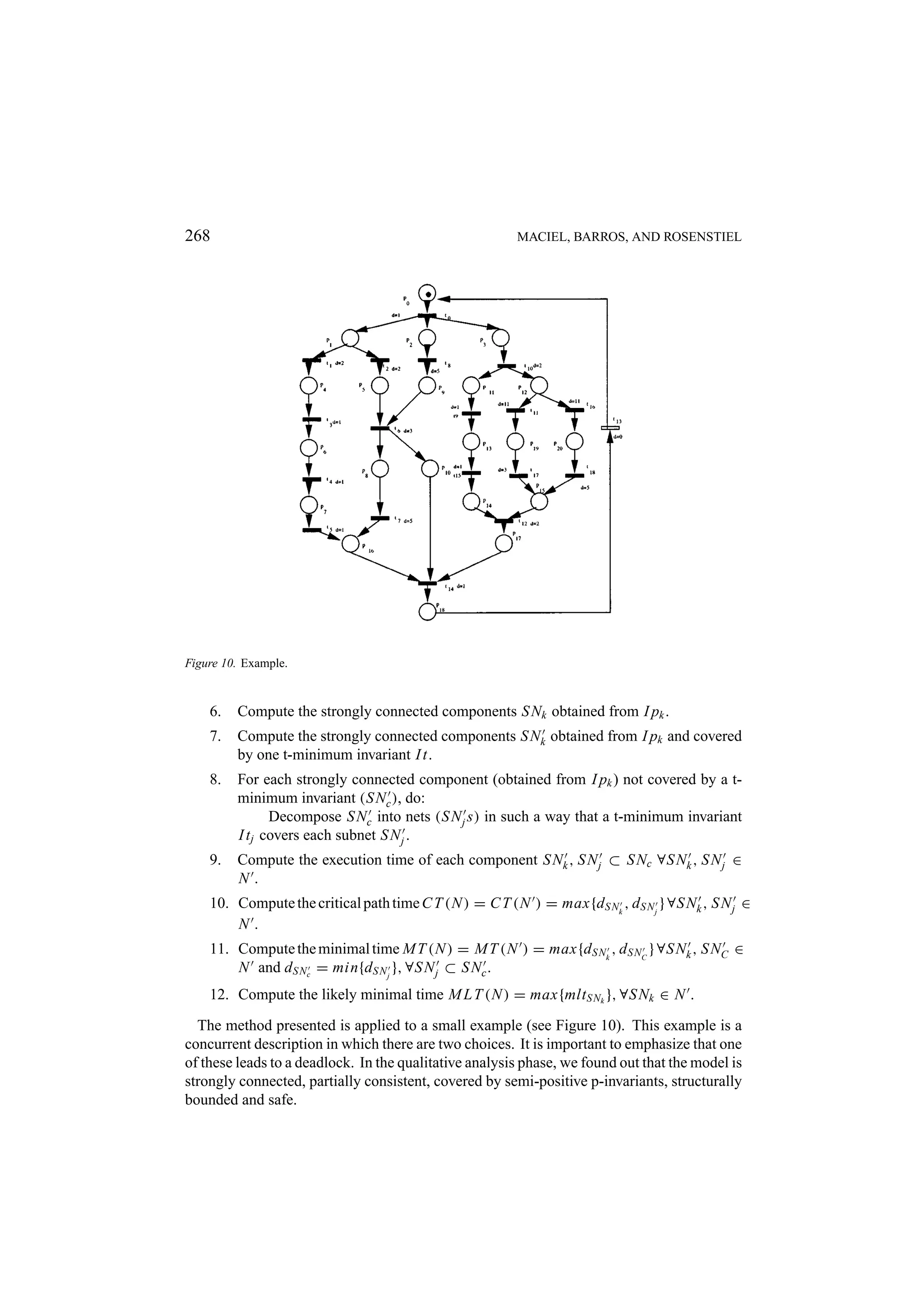
266 MACIEL, BARROS, AND ROSENSTIEL fired. We also have to eliminate from the net every transition which belongs to a choice, in the underlined untimed model, it does not model a real choice in the timed model. For instance, consider a net in which we have the following output bag related to the place pk : O( pk ) = {ti , t j }. Thus, in the underlined untimed model these transitions describe a choice. However, if in the timed model these transition have such time constraints: di and d j and d j > di , a conflict resolution policy is applied such that transition ti must be fired. After obtaining this new net (a consistent net), each sub-net obtained by each p-minimum invariant must be analyzed. In such nets, their transitions have to belong to only one t-minimum invariant. The sub-nets which cannot satisfy this condition have to be decomposed into sub-nets such that their transitions should belong to only one t-invariant. The number of sub-nets obtained has to be the minimum, or rather, the number of transitions of each sub-net in each t-invariant should be the maximum. Definition 8.3 (Shared Element). Let N = (P, T, I, O) be a net, two subnets S1 , S2 ⊂ N , a set of places P such that ∀ pz ∈ P , pz ∈ S1 , pz ∈ S2 . The set of places P is said to be a shared element if, and only if, its places are strongly connected and ∃ pm ∈ P , ti ∈ S1 , tk ∈ S2 such that ti , tk ∈ O( pm ) and ∃ pl ∈ P , t j ∈ S1 , tr ∈ S2 such that t j , tr ∈ I ( pl ). THEOREM 8.5 Let N = (P, T, I, O) be a pure strongly connected either partially consistent or consistent net covered by p-invariants without shared elements, S Nk ⊂ N a subnet obtained from a p-minimum invariant I pi and covered by one t-minimum invariant I t j , S Nc ⊂ N a subnet obtained from a p-minimum invariant I pi and does not covered by only one t-minimum invariant I t j and if ∃ pk such that #O( pk ) > 1 then l j > h i , ∀ti , t j ∈ O( pk ). The time related to the critical path of the net N is given by C T (N ) = max{d S Nk , d S N j }, ∀S Nk , S N j ⊂ N , where S N j is obtained by a decomposition of S Nc such that each S N j ⊂ S Nc is covered by only one t-minimum invariant. THEOREM 8.6 Let N = (P, T, I, O) be a pure strongly connected either partially consistent or consistent net covered by p-invariants without shared elements, S Nk ∈ N be a subnet obtained from a p-minimum invariant I pi and covered by one t-minimum invariant I t j , S Nc ∈ N be a subnet obtained from a p-minimum invariant I pi and not covered by only one t-minimum invariant I t j and if ∃ pk such that #O( pk ) > 1 then ∃l j > h i , ∀ti , t j ∈ o( pk ). Each S N j ⊂ S Nc is covered by only one t-minimum invariant, where S N j is obtained by a decomposition of S Nc . The minimal time of the net N is given by M T (N ) = max{d S Nk , d S Nc }, ∀S Nc ⊂ N such that each d S Nc = min{d S N j }, ∀S N j ⊂ S Nc . The proof of both theorems can be found in [72]. It is important to stress that the main difference among these metrics is related to the execution time of pieces of program in which choices must be considered. The computation of the minimal time related to the whole program takes into account the choice branch which provides the minimum delay. Another important measure is the likely minimal time. This metric takes into account probabilities of branches execution. Therefore, based on specific collected statis-

A PETRI NET MODEL 267 tics, the designer may provide, for each branch in the description, the probability of execution. Deﬁnition 8.4 (Strongly Connected Component Probability Matrix). Let a net N = (P, T, I, O, D), a strongly connected component S Nk ⊂ N be a branch bi related to a choice-net. SC P M(S Nk , t j ) is the execution probability of the transition t j in the strongly connected component S Nk .  0 if t j ∈ / S Nk . SC P M(S Nk , t j ): N × N → pri (0 ≤ R ≤ 1) if t j ∈ S Nk , t j ∈ bi .  1 if t j ∈ S Nk , t j ∈ bi , ∀bi ∈ S Nk . / Deﬁnition 8.5 (Probability Execution Vector). Let a net N = (P, T, I, O, D) and a strongly connected component probability matrix SC P M related to N . P E V (t j ): N → 0 ≤ R ≤ 1, #P E V (t j ) = T . Each vector component pev(t j ) = ∀S Nk SC P M(S Nk , t j ), ∀t j ∈ T . The likely minimal time related to the net N is given by M L T = max{mlt S Nk }, ∀S Nk , where mlt S Nk = d(t j ) × pev(t j ), ∀t j ∈ S Nk . d(t j ) is the lower bound time related to the transition t j and S Nk is a strongly connected component. Similar results are obtained for either partially repetitive or repetitive nets covered by p-invariants. In nets with these properties, instead of computing the t-minimum invariants we have to compute the support of the equation systems C · X ≥ 0, X = 0. The algorithm to compute the minimal time, the minimal critical path time and likely minimal time is given in the following: • Input: a net N = (P, T, I, O, D). branch probabilities bi = { pri ; t j }, ∀bi ⊂ N and ∀t j ∈ bi . • Output: the minimal time. the minimal critical path time. the likely minimal time. • Algorithm: 1. Compute the t-minimum invariants (I t) of the net N . 2. Remove from the net N the transition tl and the places pg ∈ I (tl ) or pg ∈ O(tl ), if it1 = 0, ∀I t, such that: N = (P , T , I , O ), where P = P pg , pg ∈ I (tl ) and/or pg ∈ O(tl ) and T = T tl . 3. Compute the p-minimum invariants (I p) of the net N . 4. Compute the probability execution vector (P E V ). 5. Compute the likely execution time of each component S Nk ⊂ N (mlt S Nk = d(t j ) × pev(t j ), ∀t j ∈ S Nk ).

268 MACIEL, BARROS, AND ROSENSTIEL Figure 10. Example. 6. Compute the strongly connected components S Nk obtained from I pk . 7. Compute the strongly connected components S Nk obtained from I pk and covered by one t-minimum invariant I t. 8. For each strongly connected component (obtained from I pk ) not covered by a t- minimum invariant (S Nc ), do: Decompose S Nc into nets (S N j s) in such a way that a t-minimum invariant I t j covers each subnet S N j . 9. Compute the execution time of each component S Nk , S N j ⊂ S Nc ∀S Nk , S N j ∈ N. 10. Compute the critical path time C T (N ) = C T (N ) = max{d S Nk , d S N j } ∀S Nk , S N j ∈ N. 11. Compute the minimal time M T (N ) = M T (N ) = max{d S Nk , d S NC } ∀S Nk , S NC ∈ N and d S Nc = min{d S N j }, ∀S N j ⊂ S Nc . 12. Compute the likely minimal time M L T (N ) = max{mlt S Nk }, ∀S Nk ∈ N . The method presented is applied to a small example (see Figure 10). This example is a concurrent description in which there are two choices. It is important to emphasize that one of these leads to a deadlock. In the qualitative analysis phase, we found out that the model is strongly connected, partially consistent, covered by semi-positive p-invariants, structurally bounded and safe.

A PETRI NET MODEL 269 Figure 11. Transformed net. If the system is partially consistent, it means that some of its transitions either are not able to be fired or, if they were fired, they would lead to a deadlock. The first step of the algorithm is the computation of the t-minimum invariant. The support of the t-minimum invariants are st1 = {t0 , t2 , t6 , t7 , t8 , t9 , t10 , t11 , t12 , t13 , t14 , t15 , t17 } and st2 = {t0 , t2 , t6 , t7 , t8 , t9 , t10 , t11 , t12 , t13 , t14 , t16 , t18 }. By analyzing these invariants it may be observed that the transitions t1 , t3 , t4 , t5 do not belong to any t-minimum invariant. The second step is the elimination of the transitions which do not belong to any t-minimum invariant and also the elimination of the places that are input and/or output of such transitions. The resulting net (obtained by this transformation) is presented in Figure 11. Considering the transitions of the branches of the choice (transitions t11 , t16 , t17 and t18 ), an execution probability of 0.5 was assigned. The following step is the computation of the p-minimum invariants of the transformed net. The support of the p-minimum invariants are: sp1 = { p0 , p1 , p5 , p8 , p16 , p18 }, sp2 = { p0 , p3 , p12 , p15 , p17 , p18 , p19 , p20 }, sp3 = { p0 , p1 , p5 , p10 , p18 }, sp4 = { p0 , p2 , p9 , p10 , p18 }, sp5 = { p0 , p2 , p8 , p9 , p16 , p18 } and sp6 = { p0 , p3 , p11 , p13 , p14 , p17 , p18 }. After that, the strongly connected components (Subneti ) are obtained from these invariants. Each component has the following transitions as its elements: Subnet1 = {t0 , t2 , t6 , t7 , t13 , t14 }, Subnet2 = {t0 , t10 , t11 , t12 , t13 , t14 , t16 , t17 , t18 }, Subnet3 = {t0 , t2 , t6 ,

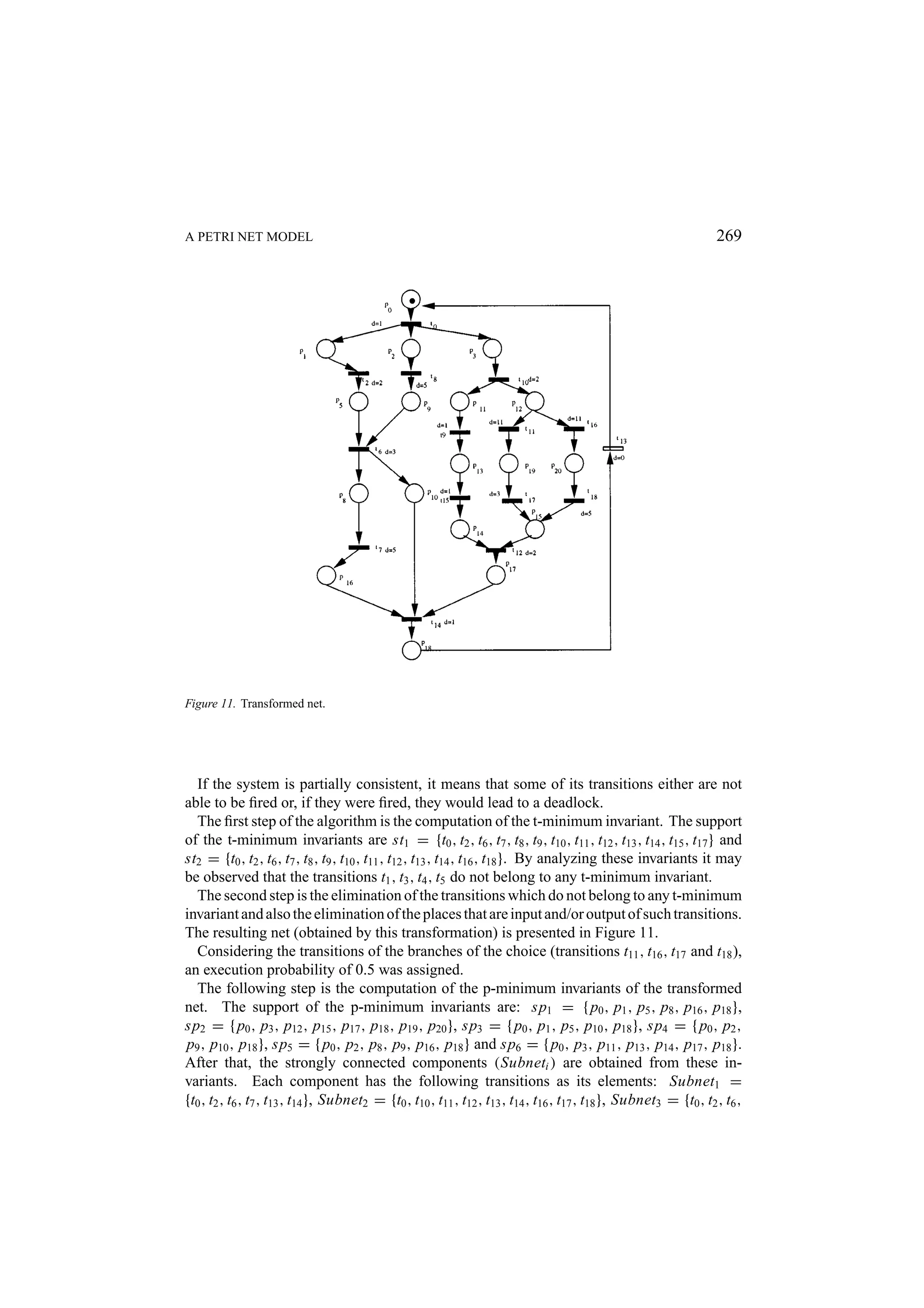
270 MACIEL, BARROS, AND ROSENSTIEL t13 , t14 }, Subnet4 = {t0 , t6 , t8 , t13 , t14 }, Subnet5 = {t0 , t6 , t7 , t8 , t13 , t14 } and Subnet6 = {t0 , t9 , t10 , t11 , t12 , t13 , t14 , t15 }. Then, the likely minimal time for each strongly connected component mlt (S Nk ) = d(t j ) × pev(t j ), ∀t j ∈ S Nk ): mlt (1) = 12, mlt (2) = 21, mlt (3) = 7, mlt (4) = 10, mlt (5) = 15 and mlt (6) = 8 is computed Each component which is not covered by only one t-minimum invariant is decomposed into subnets in such a way that each of its subnets is covered by only one t-minimum invariant. Therefore, the Subnet2 = {t0 , t10 , t11 , t12 , t13 , t14 , t16 , t17 , t18 } is decomposed into Subnet21 = {t0 , t10 , t11 , t12 , t13 , t14 , t17 } and Subnet22 = {t0 , t10 , t12 , t13 , t14 , t16 , t18 }. After that, we compute the time related to each subnet of the whole model. The resulting values are: T (1) = 12, T (21) = 20, T (22) = 22, T (3) = 7, T (4) = 10, T (5) = 15 and T (6) = 8. Then, we have C T (N ) = max{T (1), T (21), T (22), T (3), T (4), T (5), T (6)} = 22, M T (N ) = max{T (1), min{T (21), T (22)}, T (3), T (4), T (5), T (6)} = 20 and finally M L T (N ) = max{mlt (1), mlt (2), mlt (3), mlt (4) mlt (5), mlt (6)} = 21 For execution time computation in systems with data dependent loops, the designer has to assign the most likely number of iterations to the net. This number could be determined by a previous designer’s knowledge, therefore he/she may directly associate a number using annotation in the net. Another possibility is by simulating the net on several sets of samples and recording how often the various loops were executed. Such a method has been applied to several examples and compared to the results obtained by the petri net tool INA. The results are equivalents, but INA only provides the minimal time. 9. Extending the Model for Hardware/Software Codesign This section presents a method for estimating the necessary number of processors to execute a program, taking into account the resource constraints (number of processors) provided by the designer, in order to achieve best performance, disregarding the topology of the interconnection network. First, let us consider a model extension in order to capture the number of processors of the proposed architecture. The extended model is represented by the net N = (P, T, I, O, M0 , D), which describes the program, a set of places P in which each of its places ( p ) is a processor type adopted in the proposed architecture; the marking of each of these places represents the number of processors of the type p ; the input and the output arcs that interconnect the places of the set P to the transitions which represents the arithmetic/logical operations (ALUop ⊂ T ). In the extended model the number of conflicts in the net increases due to the competition of operations for processors [32]. These conflicts require the use of a pre-selection policy by assigning equal probabilities to the output arcs from processors places to the enabled transitions t j ∈ ALUop (O( p, t j ), p ∈ P ) in each reachable marking Mz . Thus, more formally: Definition 9.1 (Extended Model). Let a net N = (P, T, I, O, M0 , D) a program model, a set of places P the processor types adopted in the architecture such that P ∩ P = ∅ and

A PETRI NET MODEL 271 M0 ( p), p ∈ P the number of processors of the type p. Let a net Ne = (Pe , Te , Ie , Oe , M0 , e De , f ) the extended model such that Pe = P ∪ P , Te = T, Ie ( p, t j ) = 1 and Oe ( p, t j ) = 1, ∀t j ∈ ALUop , ∀ p ∈ P , otherwise Ie ( p, t j ) = I ( p, t j ) and Oe ( p, t j ) = O( p, t j ). M0 : N P∪P → N and De = D. Let Mz a reachable marking from M0 , f : Oe ( p, t j ) → 0 ≤ e R ≤ 1 a probability attached to each output arc Oe ( p, t j ) where ∀tj ∈T f (Oe ( p, t j )) = 1 such that Mz [t j > and p ∈ P . In such a model, the concurrence is constrained by the number of available processors (M0 ( p), p ∈ P ) provided by the designer. The main goal of the proposed approach is to estimate the minimal number of processors that can achieve best performance taking into account the upper bound of available processors already specified. Therefore, the designer, in the architecture generator, provides the number of available processors, then the execution time (C T ) is computed by reachability based methods. The following step comprises the reduction in the number of processors (M( p) = M( p) − 1, p ∈ P ) in order to compute a new execution time (C T ). If C T > C T , the necessary number of processors has been reached. This number of processors is used in the proposed method for initial allocation. The proposed algorithm to estimate the needed number of processor is: • Input: a net Ne = (Pe , Te , Ie , Oe , M0 , De , f ). e the number of available processors (M0 ( p), ∀ p ∈ P ). • Output: the optimum number of processors Mopt ( p), p ∈ P taking into account the resources constraints provided by the designer. the minimal execution time (CT) regarding to Mopt ( p). • Algorithm: 1. Compute the execution time C T (Ne ) 2. C T = C T (Ne ) 3. For each place p ∈ P , do: M( p) = M( p) − 1 Compute a new execution time C T (Ne ) if C T (Ne ) ≤ C T C T = C T (Ne ) Mopt ( p) = M( p), ∀ p ∈ P else or if M( p) = 0, ∀ p ∈ P end. The number of necessary processors can also be reached by taking into account either the speed up, the efficiency or the efficacy provided by the use of multiple processors. The gain in terms of execution time by a parallel execution of a program (Ne ) can be defined as the ratio between the execution time of Ne taking into account only one processor and the execution time concerning the use of # pr processors to execute it.

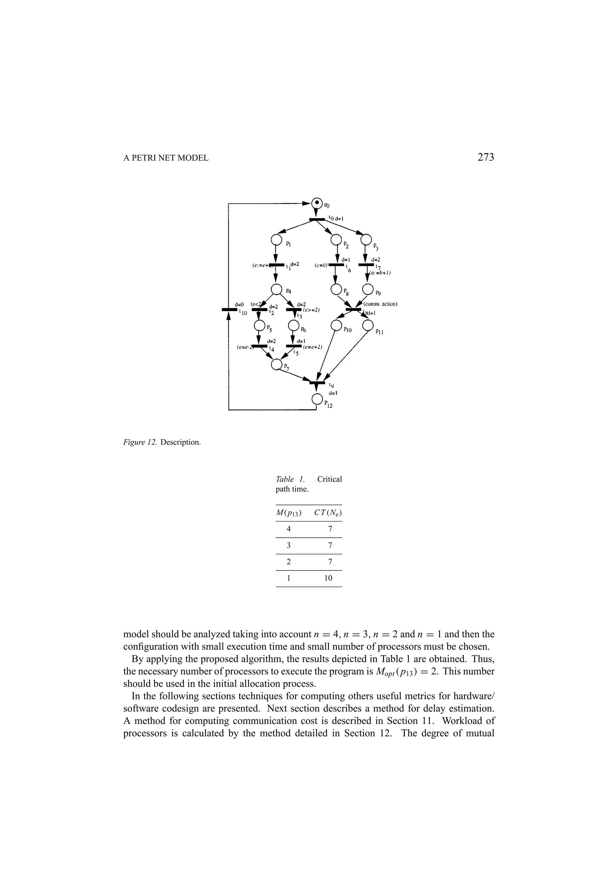
272 MACIEL, BARROS, AND ROSENSTIEL Definition 9.2 (Speed up). Let Ne be an extended model, P be a set of places representing processors of a given type adopted in the architecture, M( p), p ∈ P , be the number of processors of the type p, C T (Ne , 1) the execution time of Ne carried out by only one processor and C T (Ne , M( p)), ∀ p ∈ P , be the execution time of Ne considering M( p), ∀ p ∈ P , processors. S(Ne , M( p)) = C T (Ne , 1)/C T (Ne , M( p)), ∀ p ∈ P is defined as the speed up due to M( p)), ∀ p ∈ P , processors. The speed up of S(Ne , M( p)) provided by the use of M( p), ∀ p ∈ P , processors to execute Ne divided by the number of processors defines the efficiency. More formally: Definition 9.3 (Efficiency). Let Ne be an extended model and S(Ne , M( p)) the speed up provided by M( p), ∀ p ∈ P , processors to execute Ne . The efficiency is defined by E(Ne , M( p)) = S(Ne , M( p))/ M( p), ∀ p ∈ P . Considering the execution time C T (Ne , M( p)) as a cost measure and the efficiency E(Ne , M( p)) as a benefit, the cost-benefit relation and its inverse can be defined as the efficacy. Definition 9.4 (Efficacy). Let Ne be an extended model, E(Ne , M( p)) the efficiency, S(Ne , M( p)) the speed up, C T (Ne , 1) the execution time of Ne carried out by only one processor and C T (Ne , M( p)), ∀ p ∈ P the execution time of Ne carried out by M( p), ∀ p ∈ P , processors. E A(Ne , M( p)) = CE(Nee,M( p)) × C T (Ne , 1) = S(Ne , M( p)) × T (N ,M( p)) S(Ne ,M( p))2 E(Ne , M( p)) = M( p) , ∀p ∈ P is defined as efficacy. A small example follows in order to illustrate the proposed method. A Petri net represents the control flow of an occam program obtained by the translation method proposed in [64, 59, 61]. This net describes a program composed of three subprocesses (see Figure 12). The process P R1 is represented by the set of places PP R1 = { p1 , p4 , p5 , p6 , p7 }, the set of transitions TP R1 = {t1 , t2 , t3 , p4 , p5 }, their input and output bags (multi-sets) and the respective initial markings of its places. The process P R2 is composed of PP R2 = { p2 , p8 , p10 } as its set of places, TP R2 = {t6 , t8 }, its input and output bags and the markings of its places. Finally, the process P R3 is composed of PP R3 = { p3 , p9 , p11 } as its set of places, TP R3 = {t7 , t8 }, its input and output bags as well as the markings of its places. Each transition has the duration (d) attached to it. The extended model is represented by the net in Figure 13. The place p13 represents a processor type. Its marking represents the number of available processors. The only transitions that describe the ALU operations (t ∈ ALUop ) are interconnected in order to find out the number of functional units (ALUs—we are supposing that each processor has only one ALU) needed to execute the program and achieve best performance. These arcs are expressed by dotted lines. Due to the fact that these transitions are connected to the place p13 by an input and an output arc, for short these are represented by bidirectional arcs. Suppose, for instance, that the designer has specified, in the architecture generator, the upper bound of available processor as n = 4. Thus, the execution time of the extended

A PETRI NET MODEL 273 Figure 12. Description. Table 1. Critical path time. M( p13 ) C T (Ne ) 4 7 3 7 2 7 1 10 model should be analyzed taking into account n = 4, n = 3, n = 2 and n = 1 and then the conﬁguration with small execution time and small number of processors must be chosen. By applying the proposed algorithm, the results depicted in Table 1 are obtained. Thus, the necessary number of processors to execute the program is Mopt ( p13 ) = 2. This number should be used in the initial allocation process. In the following sections techniques for computing others useful metrics for hardware/ software codesign are presented. Next section describes a method for delay estimation. A method for computing communication cost is described in Section 11. Workload of processors is calculated by the method detailed in Section 12. The degree of mutual

274 MACIEL, BARROS, AND ROSENSTIEL Figure 13. The extended model. Table 2. Speed up, efﬁciency and efﬁcacy. Processors S E EA 1 1 1 1 2 1.4286 0.7143 1.0204 3 1.4286 0.4762 0.6803 4 1.4286 0.3571 0.5102 exclusion among processes is calculated by the method described in Section 13. The silicon area in terms of logic blocks for hardware and software implementation of each process is computed by the technique described in Section 14. 10. Delay Estimation Previous sections described methods to compute execution time (cycle time) associated to occam behavioral description translated into timed Petri nets by using the translation method proposed in [64, 61].

A PETRI NET MODEL 275 However, the method used to estimate the delay of the arithmetic and logical expressions performed in the assignments still needs to be defined. The delay of expressions is estimated in terms of the control steps needed to perform the expression. The expression execution time (delay) is given as a function composed of two factors: the delay related when performing the arithmetic and logical operations of assignments and the delay when reading and writing variables. It was assumed that operations in one expression are sequentially executed. Dex (e) = D RW (e) + D O P (e)   ∀vu ∈e D Rh (vu ) + vd ∈e DW h (vd )   if e is implemented in hardware D RW (e) =  ∀vu ∈e D Rs (vu ) + vd ∈e DW s (vd )   if e is implemented in software The variables vu and vd are the used and defined variables in the expression e.   ∀opi ∈e D O Ph (opi ) × #opi   if e is implemented in hardware D O P (e) =  ∀opi ∈e D O Ps (opi ) × #opi   if e is implemented in software 11. Communication Cost This section presents the method proposed for computing communication cost between processes by using Petri nets [69, 70]. The communication cost related to a process depends on two factors: the number of transferred bits by each communication action and how many times the communication action is executed (here referred as number of communication). Considering that we are dealing with behavioral descriptions that are translated into Petri nets, we have already defined, in each communication action, the number of transferred bits in each communication action execution. Definition 11.1 (Number of Transferred Bits in a Communication Action). N bb : nbc → N, where #N bb = T and T is the set of transitions. Each component (nbc), associated to a transition that represents a communication action, defines the number of transferred bits in the respective communication action, otherwise is zero. However, we have to define a method to compute how many times the communication action is executed the process, the communication cost for each process, the communication cost of the whole description, the communication cost between two sets of processes and finally to compute the normalized communication cost. The communication cost for each process (CC( pi )) is the product of the number of transferred bits in each communication action (N bc ) and the number of communication (N C( pi )).

276 MACIEL, BARROS, AND ROSENSTIEL Definition 11.2 (Communication Cost for each Process). Let N bc be the number of transferred bits in the communication actions and N C( pi )T a vector that represents the number of communication. The communication cost for each process pi is defined by CC( pi ) = N bc × N C( pi )T . The Number of Communication (N C( pi )) is a vector, where each component (nc( pi )), associated to a transition that represents a communication action in the process pi , is the execution number related to the respective communication action, otherwise, that is, the component vector associated to the transition which does not represent the communication action in the process pi is zero. More formally: Definition 11.3 (Number of Communication). N C( pi ): nc( pi ) → N, where: #N C( pi ) = T and T is the set of transitions. Each component nc( pi ) = max(nc X k ( pi )), ∀X k , where X k is a vector of positive integers such that either C · X = 0 or C · X ≥ 0. N C X k ( pi ): nc X k ( pi ) → N, where #N C X k ( pi ) = T and T is the set of transitions. Each vector X k is the minimum support which can be obtained by solving either C · X = 0 (in this case X k are minimum t-invariants) or C · X ≥ 0. The number of communication of an action ai (represented by a transition ti ) is the respective value obtained in the component xi for the correspondent X k . The other components, which do not represent communication actions in the process pi , are equal zero. According to the results obtained in the qualitative analysis, it is possible to choose methods to compute the number communication (N C pi ) considering the complexity of the method used. If the net (system) is consistent, first we have to compute the minimum t-invariants then the N C( pi ), ∀ pi ∈ D, are obtained. However, if the net is not consistent, but is repetitive, first the minimal support to X k , which is obtained using X in the system C · X ≥ 0, where X = 0, has to be obtained, then the N C( pi ), ∀ pi ∈ D are computed. In the case of the net not being repetitive and if it is possible to transform it into a repetitive or consistent net by inserting one transition t f such that I (t f ) = { p f } and O(t f ) = { p0 }, we apply the same method to compute X and then to obtain the N C( pi ), ∀ pi ∈ D. These places ( p0 and p f ) are well defined, because one token in the place p0 (initial place) enables the execution of the process and when one token arrives in the place p f (final place), it means that the execution has already finished. Otherwise, if it is not possible to transform the net into a repetitive or consistent one, although this system seems not to have interesting properties and even so the designer does not intend to modify it, we can compute the X and then N C( pi ) by using either the reachability graph or by solving the system C · X = M f inal − M0 , where M f inal and M0 are the final and the initial markings, respectively. However, the reader has to remember that the state equation could provides spurious solutions for some Petri net sub-classes [33]. THEOREM 11.1 Let N be a consistent net and X k a minimum t-invariant in the net. Con- sidering every minimum t-invariant in the net (∀X k ∈ N ), the maximum value obtained for each component vector is the minimum transition firing number for each transition.

A PETRI NET MODEL 277 THEOREM 11.2 Let N be a repetitive net and X k a minimum support in the net which can be obtained by using X which solves the equation C · X ≥ 0. Considering every minimum support X k in the net, the maximum value obtained for each component vector is the minimum transition firing number for each transition. The proof for both theorems can be found in [70]. The communication cost between two processes ( pi and p j ) is the product of the number of communications between the processes by the number of transferred bits in each communication action. More formally: Definition 11.4 (Communication Cost between Processes). Let N bc : nbc → N be the number of transferred bits in a communication action and N C( pi , p j ) a vector that represents the number of communication between the processes pi and p j . The communication cost between processes is defined by CC( pi , p j ) = N bc × N C( pi , p j )T . The communication execution number between two processes ( pi and p j ) is represented by a vector, where each vector component, associated to a transition which represents a communication action between both processes, defines the execution number related to the respective action. Definition 11.5 (Number of Communication Between two Processes). N C( pi , p j ): nc( pi , p j ) → N, where #N C( pi , p j ) = T and nc( pi , p j ) = min(nc( pi ), nc( p j )). In order to compute the communication cost in systems with data dependent loops, the designer has to assign the more likely number of iteration for each loop of the net. This number can be determined in two ways: the designer may either directly associate a number using annotation in the model based on previous knowledge or by simulating the model on several sets of samples in order to record how often the various loops were executed. Therefore, each component of the vector N C( pi , p j ) which represents a communication action between the processes pi and p j and that is inserted in the loop lk has to be multiplied by the more likely number of iteration (L V (lk )) of the loop lk . A similar procedure has to be taken for the vector N C( pi ). In this case, each component of the vector which represents the communication action of the process pi and which is inserted in the loop lk has to be multiplied by the more likely number of iteration (L V (lk )) of the loop lk . In the following, we present the algorithms to compute the number of communications between pairs of processes (N C( pi , p j )) and the the number of communication of each process (N C( pi )) taking into account data dependent loops. • Input: set of processes {. . . , pi , . . .}, set of loops {. . . , lk , . . .}, set of communication action (SC A = {. . . , t j , . . .}), more likely number of iteration of each loop (L V (lk )), N C( pi ) of each process.

278 MACIEL, BARROS, AND ROSENSTIEL • Output: N C( pi ) of each process taking into account the data dependent loops. • Algorithm: • For each process pi ∈ D, do: For each loop lk ∈ pi , do: For each transition t j ∈ lk , do: L V (t j ) = L V (lk ) For each loop lm ∈ pi , do: If lm ⊆ lk , do: For each transition t j ∈ SC A, do: L V (t j ) = L V (t j ) × L V (lm ) Else For each transition t j ∈ SC A, do: L V (t j ) = min{L V (t j ), L V (L m )} For each transition t j ∈ SC A, do: N C( pi , t j ) = N C( pi , t j ) × L V (t j )T • Input: set of processes {. . . , pi , . . .} set of communication action (SC A = {. . . , t j , . . .}), N C( pi ) of each process taking into account the data dependent loops, N C( pi , p j ) of each pair of processes. • Output: N C( pi , p j ) of each pair of processes taking into account the data dependent loops. • Algorithm: • For each pair of processes ( pi , p j ) ∈ D, do: For each transition tk ∈ SC A, do: If N C( pi , p j , t j ) = 0, do: N C( pi , p j , tk ) = min{N C( pi , tk ), N C( p j , tk )} The behavioral description communication cost is given by summing the communication cost between each pair of processes in the description. More formally: Deﬁnition 11.6 (Communication Cost). CC(D) = ∀( pi , p j )∈D CC( pi , p j ) In order to be able to compare distinct metric values, we have adopted two kinds of normalization: local and global normalization. The normalization refers to scaling of metric values to a number between 0 and 1. The normalization provides a possibility of combining different units, such as communication cost and mutual exclusion degree, into a single value and it also provides an absolute closeness measure between objects. Thus, we know that a closeness value between two objects of 0.95 is high, nevertheless we can not assert about the number 25 [7].

A PETRI NET MODEL 279 The global normalized communication cost between two processes is defined by the communication cost between these processes divided by the communication cost for the whole description. Definition 11.7 (Global Normalized Communication Cost). Let CC( pi , p j ) be the communication cost between processes pi and p j , and CC(D) the communication cost in the whole behavioral description. The global normalized communication cost is defined by CC( pi , p ) N CC( pi , p j ) = CC(D)j . The local normalized communication cost between two processes is defined by the communication cost between both processes divided by the summation of the communication cost for each process. Definition 11.8 (Local Normalized Communication Cost). Let CC( pi , p j ) be the communication cost between processes pi and p j , and CC( pi ) and CC( p j ) the communication cost of the processes pi and p j , respectively. The local normalized communication cost is defined by LCC( pi , p j ) = CC( pi p j )/(CC( pi ) + CC( p j )). The global normalized communication cost must also be defined for each process. This metric is defined by the communication cost related to the process divided by the communication cost of the whole description. Definition 11.9 (Global Normalized Communication Cost of a Process). Let CC( pi ) be the communication cost for each process and CC(D) the communication cost of the whole behavioral description. The global normalized communication cost of each process is defined by N CC( pi ) = CC( pi ) . CC(D) The local normalized communication cost for each process pi is defined by the communication cost of the process divided by the summation of the communication cost of processes p j s which has some communication (CC( pi , p j ) = 0). In the following we present the formal definition: Definition 11.10 (Local Normalized Communication Cost of a Process). Let CC( pi ) be the communication cost for each process pi and p j one process which CC( pi p j ) = 0. The local CC( pi ) normalized communication cost of each process is defined by LCC( pi ) = CC( p ) . ∀ p j ∈D j The algorithms below compute the the number communication between pairs of processes (N C( pi , p j )) and the communication execution number of each process (N C( pi )) taking into account the data dependent loops. 1. Compute the communication execution number for each process (N C( pi )) 2. Compute the communication cost of each process pi (CC( pi ) = N bc × N C( pi )T )

280 MACIEL, BARROS, AND ROSENSTIEL Table 3. Communication cost CC( pi , p j ). Processes CC N CC LCC p1 , p2 32 0.333333 0.333333 p1 , p3 32 0.333333 0.500000 p2 , p3 32 0.333333 0.333333 Description 96 — — 3. Compute the communication execution number between each pair of processes of the whole the description (N C( pi , p j )). 4. Compute the communication cost between each pair of processes (CC( pi , p j ) = N bc × N C( pi , p j )T ) 5. Compute the communication cost of the whole description (CC(D) = ∀( pi , p j )∈D CC( pi , p j )) 6. Compute the global normalized communication cost of each process (N CC( pi ) = CC( pi ) CC(D) ). 7. Compute the local normalized communication cost of each process (LCC( pi ) = CC( pi ) CC( p j ) ) ∀ p j ∈D 8. Compute the global normalized communication cost of each pair of processes CC( pi , p ) (N CC( pi , p j ) = CC(D)j ) 9. Compute the local normalized communication of each pair of processes (LCC( pi , p j ) = CC( pi , p j )/(CC( pi ) + CC( p j ))). Applying the proposed algorithm to the example shown in Figure 14.a, the results described in Table 3 and in Table 4 are obtained (considering that an integer is represented by 32 bits). Figure 14.b shows the net that represents the control ﬂow of the algorithm described. Table 4. Communication cost of processes. Process CC N CC LCC p1 32 0.333333 0.333333 p2 64 0.666667 1 p3 32 0.333333 0.333333

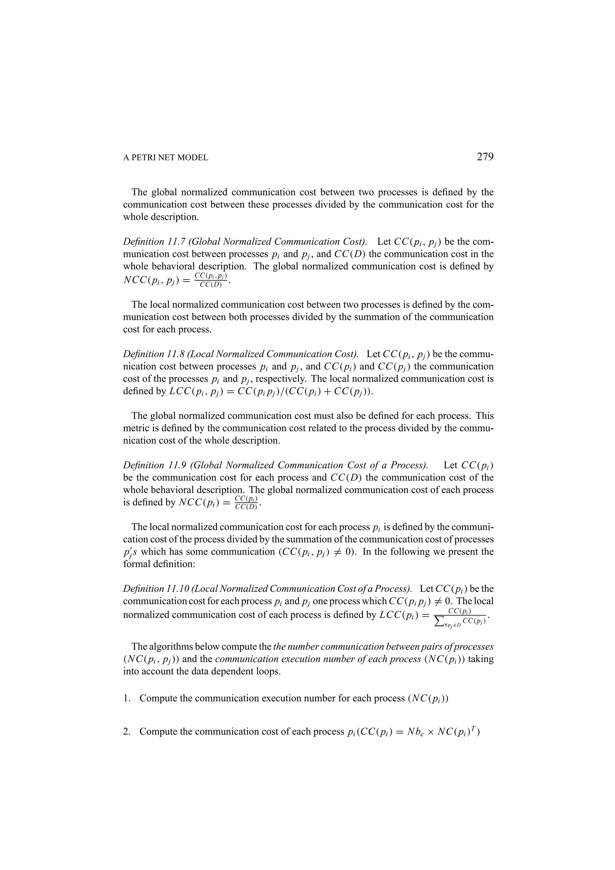
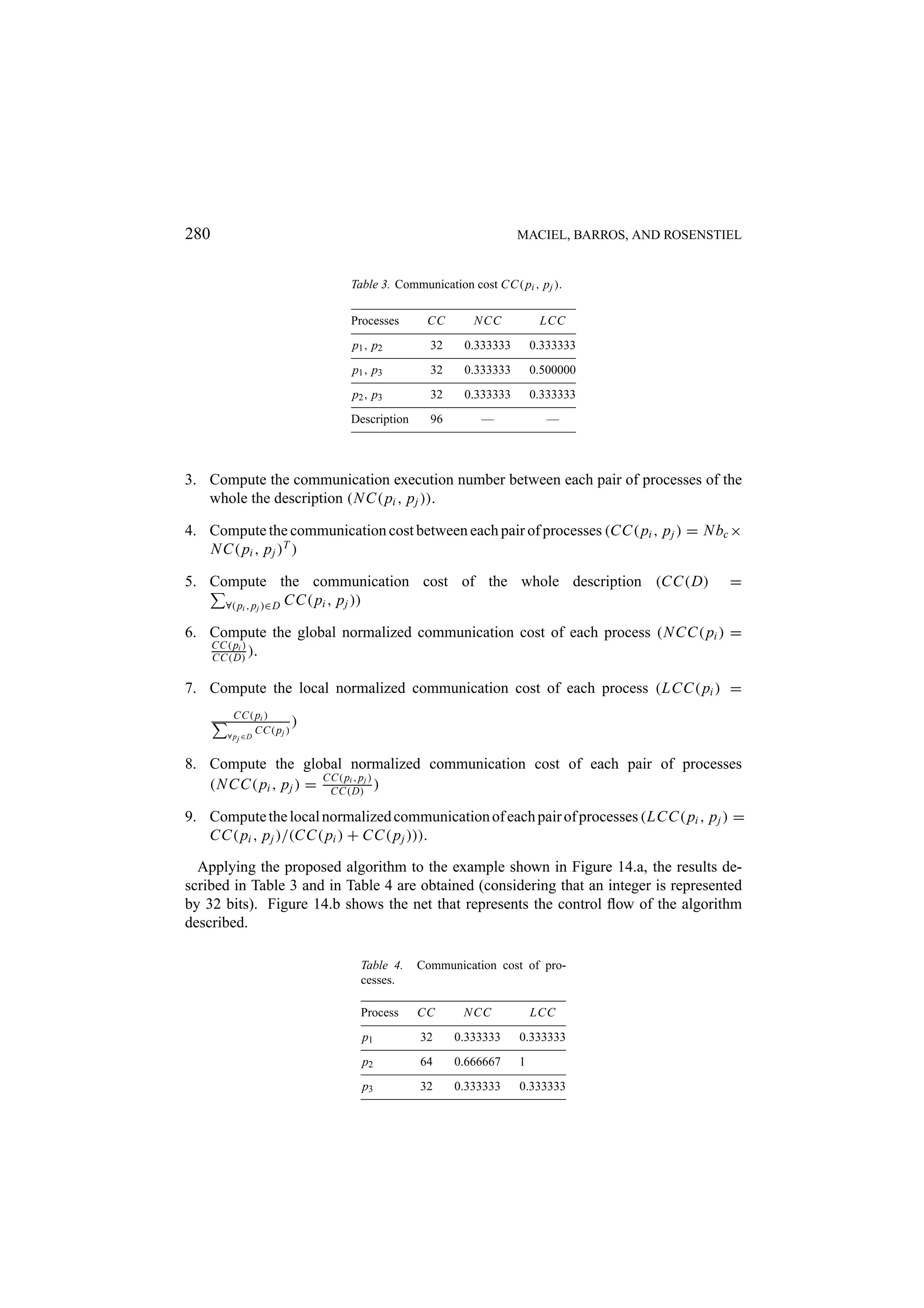
A PETRI NET MODEL 281 Figure 14. Example. It is important to stress that the algorithm proposed is based on the well known structural Petri net methods, that is, it is a formal approach that takes into account the computation of semiflows (invariants) in order to find the number of transition firings related to communication action in the processes. One common measure for quantifying communication cost is through the delay related to communication actions between processes [68, 91]. In the method proposed in this section, communication cost is calculated in terms of the amount of data transferred between processes. This approach allows one to compute the communication cost without considering assignments in a particular processor, since it is unnecessary to estimate the exact time for the communication actions. 12. Load Balancing In this section a method for computing the static load balancing among simple occam processes across processors [72] is presented. This metric is an important aspect of performing the initial allocation as well as the partitioning. The occam simple processes may be either sequential or concurrent. Parallel processes may have distinct parallelism degrees. The load balance is defined in terms of loading related to processes in the processors. For instance, if two processes pi and p y are assigned to two processors (processor K, processor L), the load balance among this pair of processors related to that specific pair of processes is defined in terms of the process loading in the processors.

282 MACIEL, BARROS, AND ROSENSTIEL The work load of one process, for instance pi , in one processor (PK ) is defined in terms of number of cycles demanded to execute such a process in the processor. Therefore, parallel processes have to be sequentialized in order to find out the execution time needed to carry out such processes. The approach used to find out the minimal execution time to carry out a process was described in Section 9. Definition 12.1 (Load). Let pi be a process and PK a processor. The work load of the process pi in the processor PK is defined by Load( pi , PK ) = N C(Pi , PK ), where N C( pi , PK ) is the sequentialized number of cycles to execute the process pi in the processor PK . The normalized loading of one process is defined in terms of the work load related to the respective process and the workload of the whole description. Definition 12.2 (Normalized Loading). Let pi be a process, PK a processor and Load( pi , PK ) the workload of the process pi in the processor PK . The normalized workload is defined by Nload( pi , PK ) = Load( pi ,PK ) where Load(D) is the description load. Load(D) The local normalized load balance for each pair of processes is defined as a function of the loading associated to each of its processes in the respective processor. Definition 12.3 (Local Normalized Load Balance between two Processes). Let pi and p j be processes and PK , PL processors. The load balance between each pair of processes related to the respective processors is defined by L L B( pi , p j , PK , PL ) = |Load( pi , PK ) − Load( p j , PL )|/(Load( pi , PK ) + Load( p j , PL )). In a similar way, the global normalized load balance metric for each pair of processes is defined as follows: Definition 12.4 (Global Normalized Load Balance between two Processes). Let pi and p j be processes and PK , PL processors. The load balance between each pair of processes related to the respective processors is defined by G L B( pi , p j , PK , PL ) = |Load( pi , PK ) − Load( p j , PL )|/Load(D), where Load(D) is the work load related to the whole description. The global normalized approach is only used if all processors have the same character- istics. The reason for this restriction is that the load related to the whole description is a function of the number of cycles necessary to execute the description in the available processor. Thus, it is more convenient to compute if considering only one type of processor. Otherwise, it has to be known in advance which part of the description is assigned to each processor. Table 5 presents the workload of each process of the example presented in the previous section. Table 6 shows the load balancing related to each pair of processes when considering their allocation on a Transputer T 800.

A PETRI NET MODEL 283 Table 5. Loading. Process Load Nload p1 39 0.196970 p2 54 0.272727 p3 110 0.555556 Description 198 — The load balance metrics used in [91] considers the work loading of a processor in terms of the average loading of the set of processors. However, the average value considered is obtained by dividing the summation of the loading of each process by the number of processors available in the architecture. This metrics, clearly, does not consider synchronization between concurrent processes. The global normalized metrics proposed in this section compares the loading related to pairs of processes and the execution time of the whole task considering synchronization and concurrent execution. On the other hand, the local normalization proposed takes into account the loading of pairs of processes. 13. Mutual Exclusion This section describes a method to compute a mutual exclusion metrics based on Petri nets [73] for use in the initial allocation and in the partitioning process as well. First of all, it is important to deﬁne clearly what we mean by mutual exclusion in the context of this work. Two processes are said to be in mutual exclusion if the execution of one implies that the other process is not executed at the same time. In this sense, either tasks which have a precedence relation (they are in a sequential fashion etc) or those whose execution excludes the execution of the others by mechanisms such as shared variables, semaphores, monitors and communication actions are said to be in mutual exclusion. If two processes are in mutual exclusion, they are less likely to reduce performance when assigned to one single processor [7, 68]. However even mutually exclusive processes could allow a certain level of concurrency. In this sections an approach to computing a mutual exclusive metrics between pairs of processes is presented. The values obtained are Table 6. Load balancing. Processes LLB GLB p1 , p2 0.161290 0.075758 p1 , p3 0.476510 0.358586 p2 , p3 0.341463 0.282828

284 MACIEL, BARROS, AND ROSENSTIEL a mutual exclusion degree between each pair of processes which are used to perform the initial allocation as well as the partitioning. As mentioned, this work deals with occam descriptions which are translated into Petri nets. Thus, the Petri net models obtained describe synchronous concurrent behaviors. It is still important to make it clear that the nets obtained are strongly connected and that only the initial place (place which is precondition to starting the firing sequences) is marked. According to our proposed translation method, the entities which represent the actions (assignment, stop, skip etc) of the occam processes are transitions. The places represent pre-conditions and post-conditions related to the transition firing. The pre-condition which enables the evaluation of the function y and the respective value assignment to the variable x is represented by the place pre-condition. The function execution is represented by the transition action and the post-condition is represented by the place post-condition. When one token is stored in the post-condition place, it means that the local state representing the evaluation of the function y (execution of the action) has already been reached. Using the serial-places reduction rule, this net is directly transformed into a place. Thus, the obtained place (activity) represents the whole activity, that is, the pre-condition, the action and the post-condition. Mutually exclusive statements in the model (net obtained from the occam description by applying the proposed translation method) by analyzing the minimum p-invariants. Two places pk and pr are in mutual exclusion if, and only if, they are never simultaneously marked. We define M E X ( pk , pr ) as a function which represents the mutual exclusion between two statements (places) in pairs of processes (constituted by places, transitions and the respective relations) of one description. Thus, if these places are in mutual exclusion, (m( pk ) = 0) ∨ (m( pr ) = 0) (place markings). Definition 13.1 (Mutual Exclusion between Statements). Let ( pk , pr ) be a pair of statements of two processes in one description, respectively.  1 if pk and pr are M E X ( pk , pr ) = in mutual exclusion  0 otherwise To analyse whether two places (statements) are in mutual exclusion, first we have to compute the minimum p-invariants (I p ’s) and then multiply each one by the initial marking of the net (M0 ). If the obtained product is I p × M0 = 1, the places which are support to this T i T minimum p-invariant are in mutual exclusion. Then we analyze, for each pair of processes ( pri , pr j ), whether each pair of places ( pk ∈ pri , pr ∈ pr j ) is in mutual exclusion. If it is, we make M E X ( pk , pr ) = 1, otherwise we make M E X ( pk , pr ) = 0. In order to perform the initial allocation and the partitioning, it is important to define a metrics which provides a mutual exclusion degree for each pair of processes ( pri , pr j ) of the description. Although they are pairs of processes in which the processes are in mutual exclusion, they could have distinct mutual exclusion degrees. For example, consider two pairs of processes ( pri , pr j ) and ( pr y , pr z ) in which the processes are in mutual exclusion.

A PETRI NET MODEL 285 If between the processes pri and pr j there is only one small piece of their description which is mutually exclusive, while between the processes pr y and pr z there are several regions which are in mutual exclusion, obviously these pairs of processes have distinct mutual exclusion degrees. L M E( pri , pr j ) is defined as a local normalized metrics which represents the mutual exclusion degree between two processes pri and pr j . Definition 13.2 (Local Normalized Mutual Exclusion Metric between Processes). Let pk and pr be statements of two processes pri and pr j of a description D. L M E( pri , pr j ) = pk ∈ pri , pr ∈ pr j M E X ( pk , pr )/(| pri | × | pr j |), ∀ pk , pr , where pri , pr j ∈ D and (| pri | × | pr j |) represents the total number of pairs of places (statements) between those processes. L M E( pri ) has also been defined as a local normalized mutual exclusion degree related to one process ( pri ). The local normalization is due to the fact that only other processes ( pr j ) which have pk ∈ pri , pr ∈ pr j M E X ( pk , pr ) = 0 have been considered. Definition 13.3 (Local Normalized Mutual Exclusion Metric for One Process). Let pk and pr be statements of processes pri and pr j of a description D. L M E( pri ) = M E X ( pk , pr )/( | pri | × | pr j |), ∀ pk ∈ pri , ∀ pr ∈ pr j , ∀ pr j ∈ D if, and only if, M E X ( pk , pr ) = 0, ∀ pk ∈ pri , ∀ pr ∈ pr j . (| pri | × | pr j |) represents the total number of pairs of places (statements) between those processes. In order to reduce the complexity to compute the mutual exclusion degree, a set of reduction rules [37, 38] is applied to the net, then the p-invariants related to the reduced net are computed. We have applied two reduction rules: parallel-places reduction and serial-places reduction1 In the reduced net, the places which represent a set of places in the original model are attached with indexes that provide the number of places they represent in the original net. This approach has shown interesting results in terms of computation time reduction. The algorithm to compute the mutual exclusion degree between pairs of processes is described below: 1. Apply the reduction rules to the original net. As a result, a reduced net is obtained along with the set of index related to the places (RPS-reduced place set). 2. Compute the p-invariants of the reduced net. 3. For each pair of process ( pri , pr j ), do: For each pair of places ( pk , pr ) belonging to both processes, do: If the pair of places ( pk , pr ) belongs to one p-invariant do: M E X ( pk , pr ) = 1 and smex( pri , pr j ) = smex( pri , pr j ) + (M E X ( pk , pr ) × r ps( pk ) × r ps( pr )) L M E( pri , pr j ) = smex( pri , pr j )/(| pri | × | pr j |).

286 MACIEL, BARROS, AND ROSENSTIEL Table 7. Mutual exclusion degree of the pairs of processes. Processes LME p1 , p2 0.5 p1 , p3 0.15 p2 , p3 0.3 4. For each process pri , do: For each process pr j , do: If smex( pri , pr j )! = 0, do: smex( pri ) = smex( pri , pr j ) L M E( pri ) = smex( pri)/( | pri | × | pr j |) 2 The results obtained for the toy example shown in Section 11 are presented in Table 7 and Table 8. It should be stressed that previous works devoted to the mutual exclusion analysis have only considered the qualitative point of view [88, 87]. Nevertheless, when considering process allocation and hardware/software partitioning, it is important to quantify such a property. Although such an approach has been based on the well known p-mutex concept, this method extends it since a quantiﬁcation of statements is provided. The method proposed in [68] describes a method for analyzing precedence relation between pairs of processes in order to perform process allocation, however it does not take into account exclusion related to choice-branches. The method proposed in this section considers both, causal precedence relation and statements in distinct branches of choices. 14. Estimating Area Area and delay estimation plays an important role when the design process is started at a high level of abstraction in order to obtain optimal or near optimal solutions. An important issue when deﬁning an estimation algorithm is the tradeoff between accuracy and the computational cost. High accuracy levels are only obtained if the model adopted Table 8. Mutual exclusion degree of processes. Process LME p1 0.230769 p2 0.357143 p3 0.214286

A PETRI NET MODEL 287 incorporates several aspects of the design. On the other hand, simple models are executed quickly and are easy to develop, but they may not provide the accuracy level required for the design. In general, at a high level of specification, the designer needs to make choices between design alternatives and observe a compromise between accuracy and complexity of the adopted model. In this case, fidelity is the key quality desired of the algorithm. If an algorithm estimates values for two different designs and the values obtained in the implementation have a comparative relationship to each other, the estimator correctly compares the implementations [9]. 14.1. Software Model This section describes the method proposed to estimate the process (behavioral description) size. Such an estimate may be divided in terms of program size and data memory size of a given behavioral description. First of all, however, the software model is described in order to perform the estimates. A software implementation of a behavioral description is obtained by compiling it into the instruction set of the processor considered in architecture. The variables are assumed to be mapped to the memory associated to the processor. Concurrent behavior, when implemented in a single processor, may be interleaved and the communication has to be implemented by shared location (channels emulation) in the memory. If two behavioral pieces of description are allocated to two different processors, we have been used channels as the communication model. Two approaches can be used for software estimation. The first, compiles the behavior into a processor model. The second approach translates the description into a generic model. The generic model estimation provides less accurate values due to the fact that generic instruction set represents only a portion of the processors instruction set. However, on the other hand, different compilers and estimators are not needed for each processor type. The generic model estimator computes the metrics based on the generic instructions and the processor’s technology files [9]. Generic instruction set may consist of five sub-sets representing arithmetic/logical operation, move/load and store operations, conditional jumps, unconditional jumps and procedure call instructions. The processor’s technology files provide information about the number of cycles and code-size for the generic instructions. These files can be obtained from the timing and size information of the processor’s instruction set. The area estimates is obtained from the generic instructions and the processor’s technology file (see Figure 15). Although generic instructions seem to be the best choice when considering the aspects described previously, so far only Transputers have been taken into account in the computer architecture. Therefore, the estimates will be much more accurate when considering the software area and delay indexes given by the manufacturer. This is the software model adopted to be used in the context of this work. Taking into account a behavioral description (process), the process software area is given in terms of behavior and variable areas:

288 MACIEL, BARROS, AND ROSENSTIEL Figure 15. Estimation model. Definition 14.1 (Software Process Area). Let ASb ( pi ) be the process behavior area and ASr w ( pi ) the read/write variables area related to the process pi . AS( pi ) = ASb ( pi ) + Asr w ( pi ) is defined as the software process area, where ASb ( pi ) = ASal ( pi ) + Ashls ( pi ), where ASal ( pi ) represents software area of arithmetic expressions and AShls ( pi ) is the area of occam high-level combiners. 14.2. Hardware Model This section describes the design model for hardware estimation. The purpose of the hardware model is to allow for hardware area and delay estimation. For a given high-level behavioral description, the hardware design can be divided into three classes of functional blocks: data-paths, local controllers and high-level constructor control. The high-level constructor control consists of circuits implementing the control of the description language. Figure 16 shows these three classes considering a high level description. The generic hardware units set is defined in the following: Definition 14.2 (Generic Hardware Units). Let D be a behavioral description. Let x: = e be an assignment of the evaluation of the expression e to the variable x, ch ? x and ch ! e the input and output primitive processes, respectively. Let STOP represent the deadlock process and SKIP be a silent action. IF is a conditional constructor, WHILE represents a loop command, SEQ denotes the sequential construction of processes, PAR stands for parallel composition and ALT represents alternation. OCS = {x: =

A PETRI NET MODEL 289 Figure 16. Hardware model. e, ch ? x, ch ! e, STOP, SKIP, IF, WHILE, SEQ, PAR, ALT} defines the set of occam statements and HLC: ocs → hlc defines a set of control circuits that implements the occam high level statements. Let OP be a set of arithmetic/logical statement (arithmetic/logical operations), D P: op → dp be a set of data-path circuits for the arithmetic/logical statements and LC: op → lc a set of local control circuits for the arithmetic/logical statements. GHU(D) = {HLC, LC, DP} is defined as the generic hardware units set of a given description D. Given a process pi , the hardware process area in terms of data-path, local-control and high-level-control circuits is defined as: Definition 14.3 (Hardware Process Area). Let AHop ( pi ) be the summation of the available functional units area that may carry out each arithmetic/logical operation, AHr w ( pi ) be the area concerning read/write variables, AHm ( pi ) be the multiplexers area, AHlc ( pi ) be the local control area and AHhlc ( pi ) be the control circuits area for high level statements. AH ( pi ) = AHop ( pi ) + AHr w ( pi ) + Am ( pi ) + AHlc ( pi ) + AHhlc ( pi ) is defined as the hardware area for implementing the processes pi . 14.3. High-Level Constructor Hardware Area Estimation This section presents a method for estimating hardware area of high-level controllers. The proposed hardware implementation of Petri nets assigns one D flip-flop, AND and OR gates to every place in the net. Transitions are implemented by using AND gates. Figure 17 shows the hardware implementation for each Petri net component: place, marked-place and transition. Hardware implementation of places considers that all flip-flops are cleared at power- ¯ up. Places with initial marking have inputs (NOR gate) and output inverted ( Q). The

290 MACIEL, BARROS, AND ROSENSTIEL Figure 17. Hardware implementation of Petri components. feedback around each flip-flop keeps its token and a previous synchronous reset feedback to all preceding flip-flops (feedback from next stage) to clear tokens as a transition fires (see Figure 17.a, b). As a transition fires only when all input conditions are satisfied, it is implemented by AND gates when there exists more than one input. If a transition has more than one output place, the feedback to its input place is implemented also by AND gate. The inputs of such an AND gate come from the inputs of the flip-flops that implement the output places (feedback to previous stage). Taking into account the foregoing models, area estimates of places and transitions for hardware implementation are given below. Definition 14.4 (Place Area Estimates). Let N = (P, T, I, O, D) be a net and p j ∈ P be a place. Let FDA be the flip-flop D area, A A be a two input AND gate area and OA be a two input OR gate area. The hardware area for hardware implementation of a place p j is estimated by AHpl ( p j ) = FDA + A A × |O( p j )| + AO × |I ( p j )|, where |I ( p j )| and |O( p j )| represent the number of input and output transitions of the place p j , respectively.

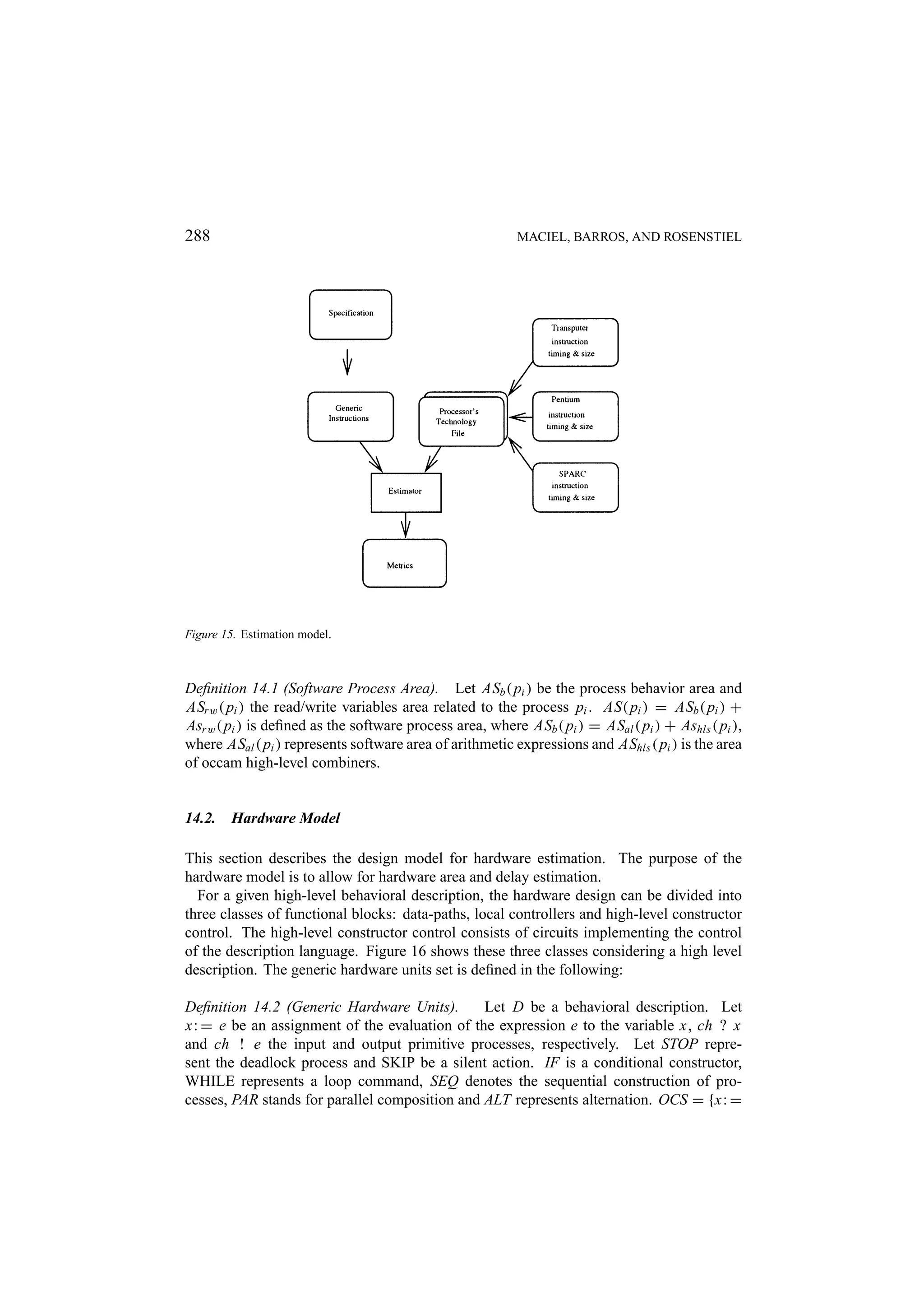
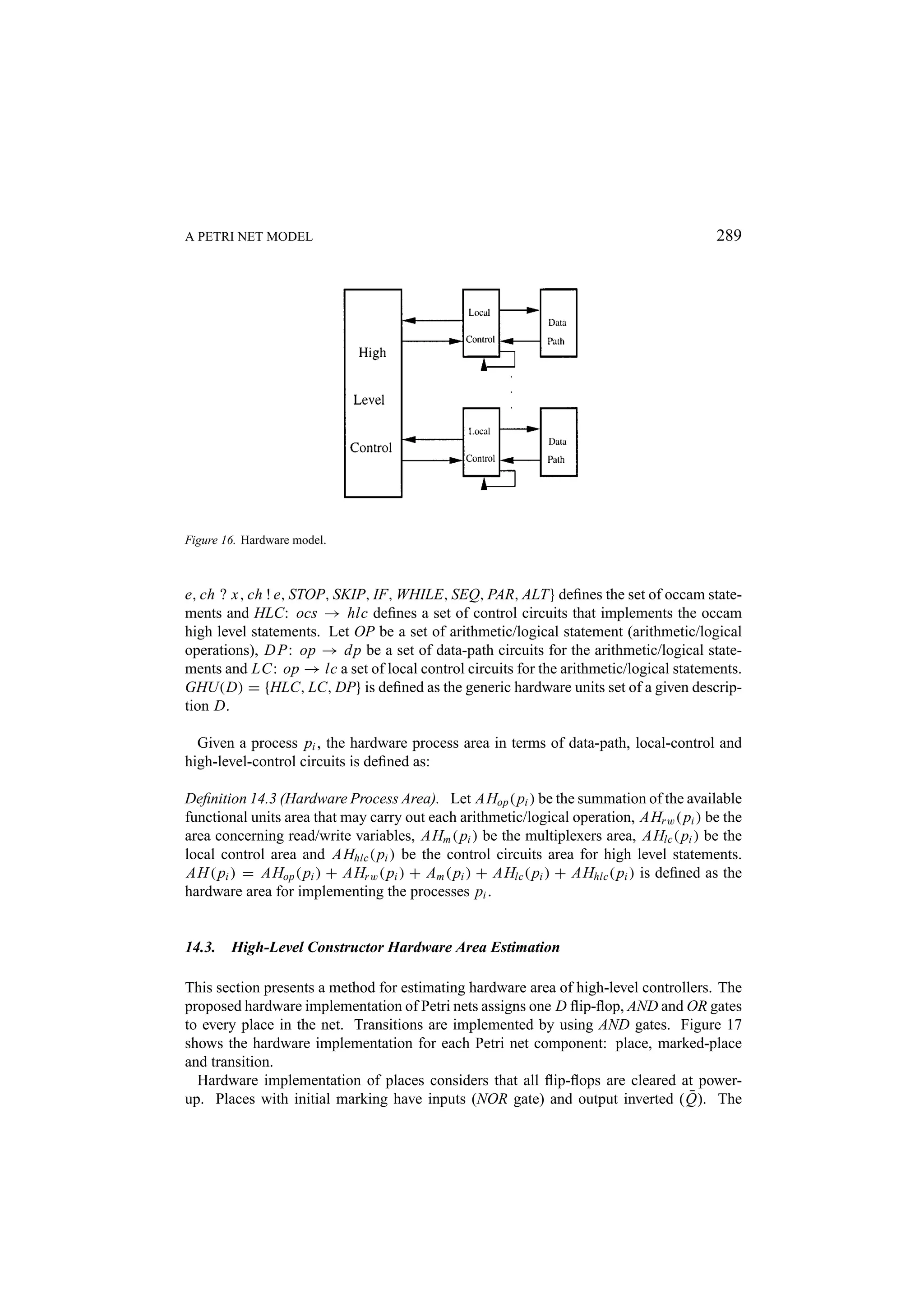
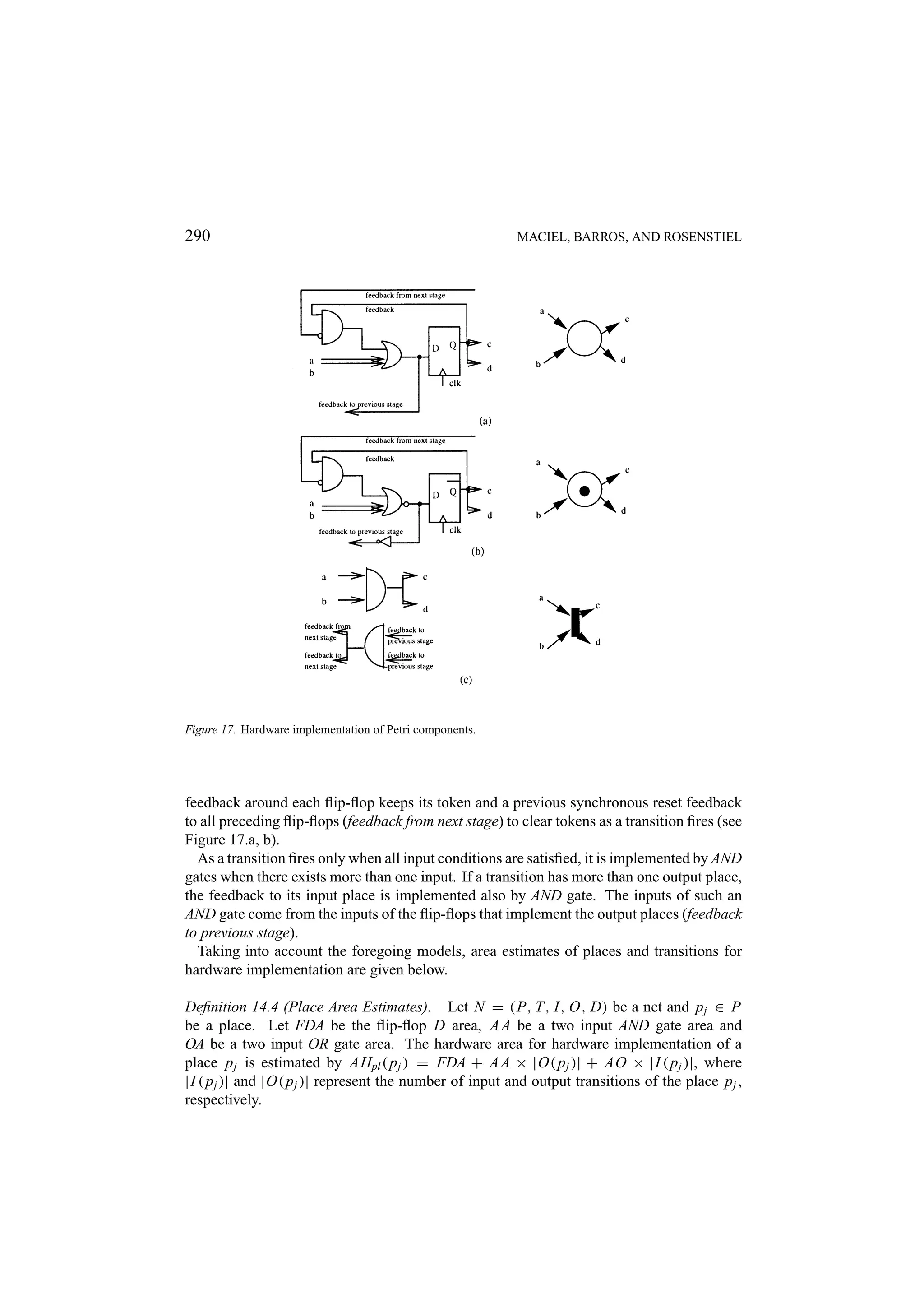
A PETRI NET MODEL 291 Definition 14.5 (Transition Area Estimates). Let N = (P, T, I, O, D) be a net and ti ∈ T be a transition. Let |I (ti )| and |O(ti )| be the number of input and output places of the transition ti , respectively. Let A A be a two input AND gate area. The hardware area for the implementation of a transition ti is given by AHtr (ti ) = Ait (ti ) − Aot (ti ), where: A A × (|I (ti )| − 1) if |I (ti )| > 0 Ait (ti ) = 0 if |I (ti )| = 0 and A A × (|O(ti )| − 1) if |O(ti )| > 0 Aot (ti ) = 0 if |O(ti )| = 0 The area related to high-level control of a behavioral description described by a Petri net is defined in terms of the area of its places and transitions. Definition 14.6 (High-Level Control Area). Let N = (P, T, I, O, D) be a net representing a behavioral description prk , AHpl ( p j ) be the hardware area for a place p j ∈ P and AHtr ti be the area for a transition ti ∈ T . The area related to the high-level control is defined as AHhlc ( prk ) = pj ∈P AHpl ( p j ) + ti ∈T AHtr (ti ). 14.4. Local Controller Area Estimation This section presents the approach adopted for estimating the local hardware control area. Local hardware controllers are hardware units that provide the step sequence required to carry out the all operations within an arithmetic/logical expression in a process, or rather, it is not related to the occam high-level constructors. Hence, a local controller area has to be estimated for each transition representing the evaluation of an arithmetic/logical expression. If this transition was obtained by reduction, the number of transitions reduced representing arithmetic/logical expressions (replication number) has to be considered. Therefore, a number of local controllers equal to the replication factor should be taken into account. Thus, the local controller area of the expression associated to such a transition is estimated as the area needed to implement one controller times its replication factor. There are several methods for implementing a sequential hardware controller. These methods include the delay element method, sequence counter method and the approach based on ROM implementation. The method taken here is the ROM based method [9]. The local controller is synthesized as a finite state machine implemented with a state register and a ROM (see Figure 18). The size of the state register depends on the number of states required to execute every operation within an assignment. The number of bits of the state register is equal to log2 ∀ej ∈ pri , ∀opi ∈ej #opi × D O Ph (opi ), where #opi : opi → N is the number of occur- rence of the operator opi within an arithmetic/logical expression e j , OPS( pi ) = {op0 , . . . , opk , . . . , opn } is the set of operations of the arithmetic/logical expression e j of a process

292 MACIEL, BARROS, AND ROSENSTIEL Figure 18. Local controller. pri and D O Ph (opi ) is the delay (in clock cycles) to carry out the operation opi . The state register inputs enable the execution (step sequence) of the operations. The state register outputs inform when the local final state has been reached. The local final state represents a given condition which states the execution of an assignment. With respect to the ROM size, it is assumed that the word-width is equal to the number of registers plus the number of functional units plus the number of multiplexers (two-to-one multiplexer type is assumed to be the adopted model). The number of words of the ROM is defined as the number of steps required to carry out the expression. It has been assumed that operation within an arithmetic/logical expression is sequentially executed, that is, only one operation is executed at a time. Therefore, the number of words needed to implement the ROM is estimated at ∀ej ∈ pri ∀opi ∈ej #opi × D O Ph (opi ). Definition 14.7 (Local Hardware Control Area). Let N S = { pr0 , . . . , pri , . . . , prn } be a set of simple processes, e j ∈ pri be an arithmetic/logical expression and OPS( pri ) = {op0 , . . . , opk , . . . , opn } be the set of operations ∀e j ∈ pri and D O Ph (opi ) be the delay (in clock cycles) needed to carry out the operation opi . Let #V S(e j ), ∀e j ∈ pri , ∀ pri ∈ N S be the number of registers within the expression e j (V S(e j ) is the set of all distinct variables defined and used within the expression e j ). Let FUN( pri , OP TYPE) be the functional unit number of the type OP TYPE related to a process pri . Let M N ( pri ) be the number of multiplexers. The local controller area (number of bits) is estimated as AHlc (N S) = ( ∀ pri ∈N S (( ∀ej ∈ pri #V S(e j ) + ∀OP TYPE∈OPS FUN( pri , OP TYPE) + M N ( pri )) × ( ∀ej ∈ pri ∀opi ∈ej #opi × D O Ph (opi )) + log2 ∀ej ∈ pri ∀opi ∈ej #opi × D O Ph (opi ))) × AHb , where AHb is hardware area for implementing one bit. 14.5. Data-Path Estimation This section describes a method for estimating the data-path area of a given behavioral description. The data-path circuit consists of registers, functional units and multiplexers. It was sup- posed that each assignment with more than one arithmetic/logical operation is implemented

A PETRI NET MODEL 293 Figure 19. Data-path model. in such a way that each operation is executed. Therefore, a model is presented in Figure 19 as a typical data-path which is used in our approach. In the data-path model used, latches are inserted at the input and output ports of functional units in order to improve performance and versatility. 14.5.1. Functional Unit Area The functional-unit area of a process is related to the area of ALU, adder, multiplier etc needed to carry out arithmetic/logical operations of the assignments in a process. If the designer knows the functional unit types that he/she has available in advance, they may adopt functional-unit area related to one that provides the greatest suitability degree (max{S( pi , FU j )}, ∀FU j ). Nevertheless, this aspect may only be considered if a functional-unit constraint list was provided by the designer, otherwise, the areas related to functional units that may execute each arithmetic/logical operation type of the expression must be considered without taking into account the suitability degree. Another aspect that has to be taken into account is the possible functional unit sharing. This aspect is very much simpliﬁed when dealing only with simple processes. In this case, it has been assumed that each operation within an expression is performed sequentially and that only one functional unit for each type of operation is used. It is important to highlight that arithmetic/logical operations such as summation, subtraction etc could be executed by the same functional units, and thus they could be considered as being of the same type. However a better estimate needs to be provided when considering more complex processes such as boxes and sets of simple processes. Such estimates should take into

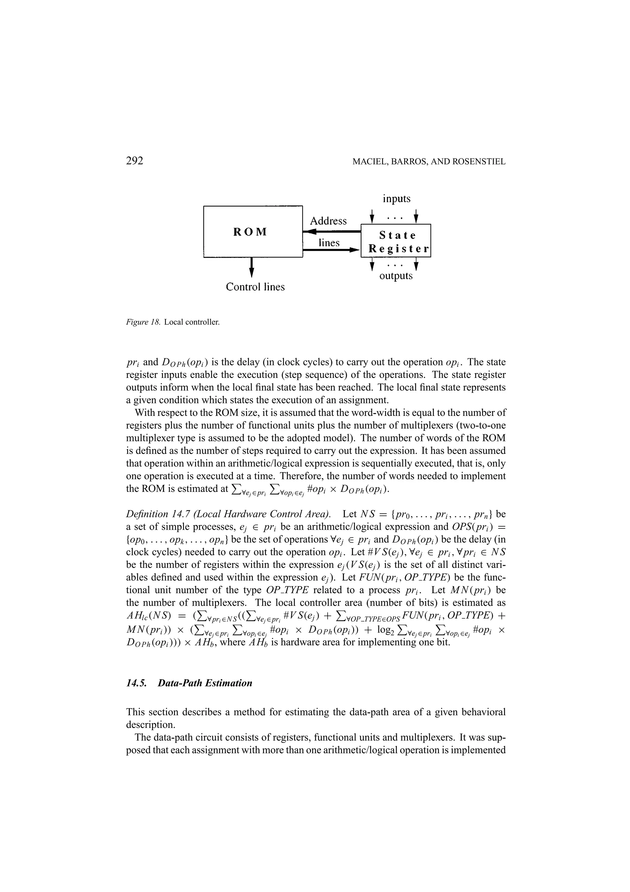
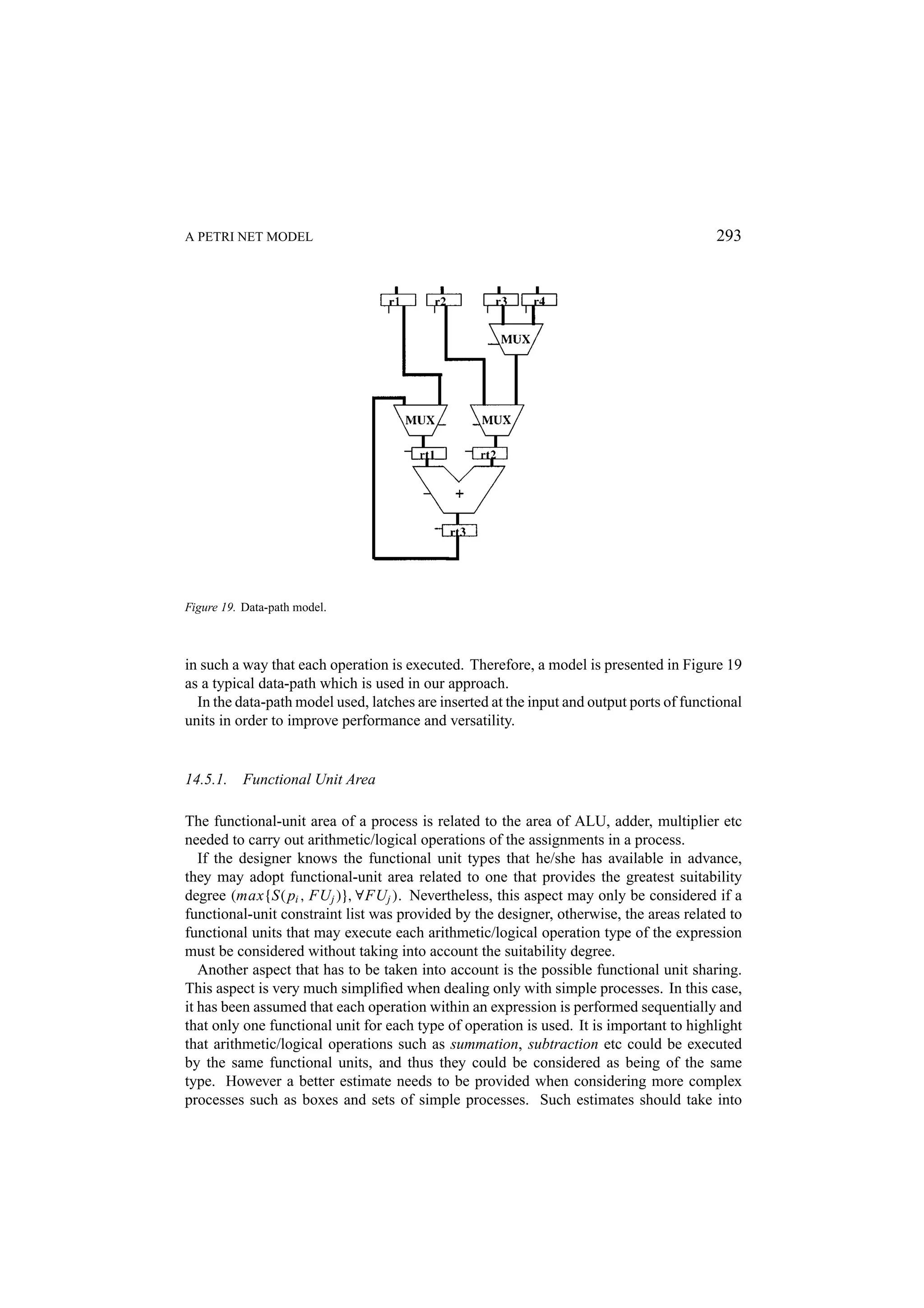
294 MACIEL, BARROS, AND ROSENSTIEL account possible resource sharing of a model chosen to carry out a set of processes or even a piece of specification described by a box. The first step when calculating the area for functional units is to determine the number of functional units needed to execute a given behavioral description. The method adopted provides an upper bound for each operation type based on the precedence relation between operators of the same type within a box or in a set of processes. In order to estimate this bound, the behavioral description is analyzed in terms of a causal precedence relation of operators in such a specification, that is, either operators which are combined to be executed in sequential fashion, the ones that have a causal relation due to communication, or the ones that are in mutual exclusion due to shared variables or semaphore implementation. Shared variable and semaphore implementation is beyond the scope of the present method, since occam has been adopted as a specification language and the communication is represented by synchronous actions. Nevertheless, it is important to stress that the method proposed is able to consider mutually exclusive statements for this kind implementations. Before a formal description of such a method, let us provide an overview of it by considering a small example: INT a,b,c,d: SEQ PAR b:b+1 a:a+1 c:=c+d The Petri net model obtained from this program is presented in Figure 20. However, a closure (t5 ) is applied to this net in order to make it strongly connected. The causal precedence relation can be analyzed by means of p-minimum invariants (I Pi ) [73]. The first step of the method is to compute the number of adders needed to carry out the description is the calculation of invariant supports. As a result, the following supports were found: (I P0 ): S P0 = { p0 , p1 , p3 , p5 , p6 } (I P1 ): S P1 = { p0 , p2 , p4 , p5 , p6 } After this, the transition-paths have to be computed. The result is provided below: T P0 = { t0 , t1 , t3 , t4 } T P1 = { t0 , t2 , t3 , t4 } In order to calculate the functional unit upper bound number needed to execute the description, the minimal number of transition-paths has to be found. These paths should

A PETRI NET MODEL 295 Figure 20. Net Nb . cover the transitions of the net of a given type (summation) that can be carried out by the related functional units (adder). For this example, two transition-paths are needed to cover the transition set T S(Nb , sum). T S(Nb , sum) = { t1 , t2 , t4 } Thus, the functional unit number obtained is equal to 2. After having this informal explanation, let us approach it formally. Considering a set of processes represented by a net set N S (each process is represented by a net S Ni ), the transition of a given type related to this set of processes is represented by the finite set T S(N S, OP TYPE). Definition 14.8 (Type Transition Set). Let N = (P, T, I, O, M0 , D) be a strongly connected net covered by p-invariant and T C A ⊆ T be a set of communication transition j (actions). Let S Ni = (Si , Ti , Ii , Oi , M0 , Di ) and S N j = (Sj , Tj , I j , O j , M0 , D j ) be i two nets representing processes where Si , Sj ⊆ P, Si ∩ Sj = ∅ and Ti , Tj ⊂ T and Ti ∩ Tj = ∅ iff ∃ tk ∈ Ti , Tj , T C A. Let N S = {S Nh , . . . , S Nl , . . . , S Nn } be a finite net set. T S(N S, OP TYPE) = {te , . . . , tk , . . . , tr } is defined as a set of transitions of a given type related to a net set N S.

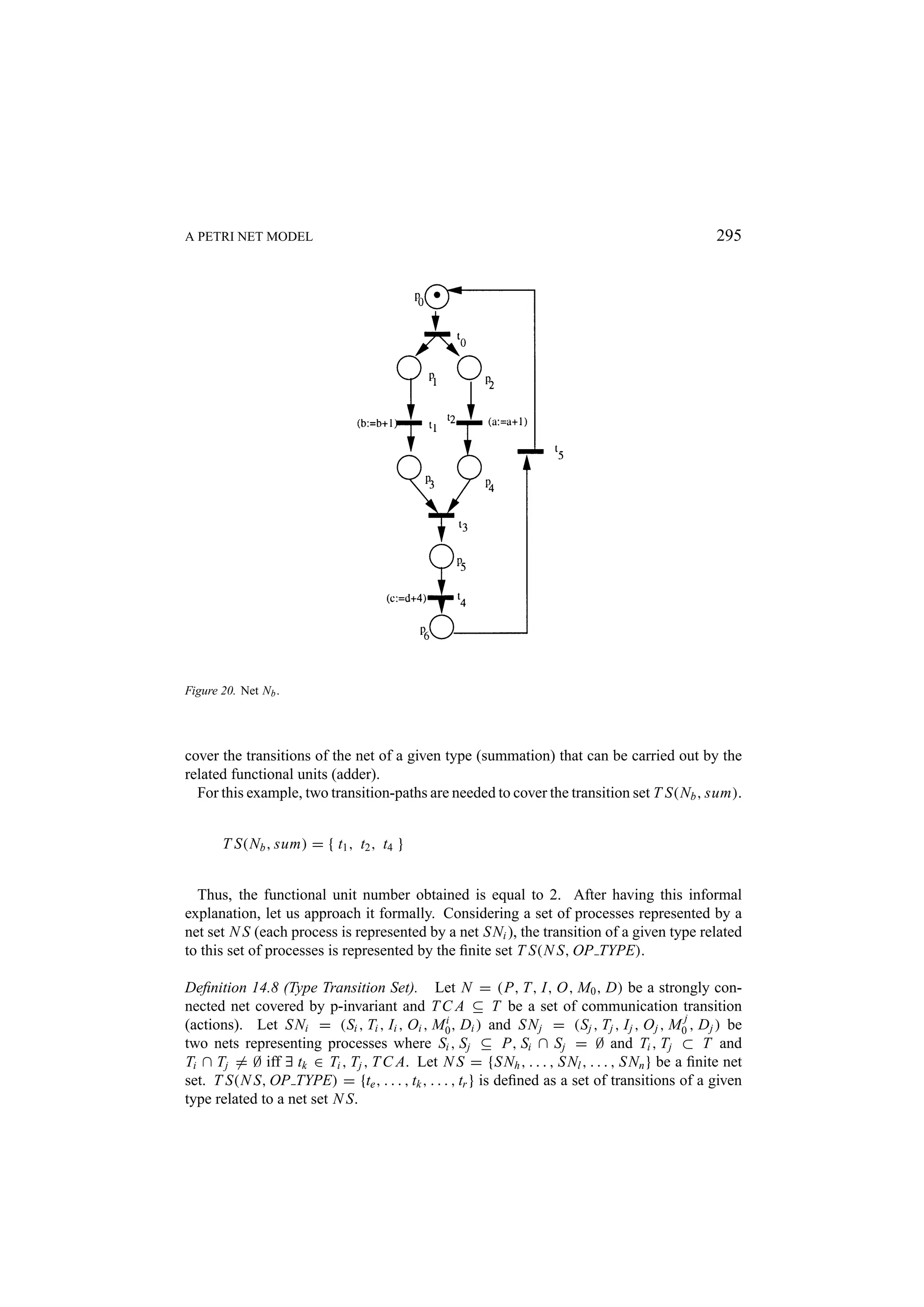
296 MACIEL, BARROS, AND ROSENSTIEL The set T S(N S, OP TYPE) can be represented by a vector T SV (N S, OP TYPE). The formal definition is given below: Definition 14.9 (Type Transition Vector). Let N = (P, T, I, O, M0 , D) be a net and T S(N S, OP TYPE) be a set of transition of the type OP TYPE for a given net set N S. 1, if type (ti ) = OP TYPE T SV (N S, OP TYPE): T → 0, otherwise defines a vector that represents the set T S(N S, OP TYPE), where ti ∈ T . For a given strongly connected net N covered by p-invariants, let us consider a subnet S Ni ⊆ N generated by a p-minimum invariant represented by a vector I Pi . The transition- path-matrix of such a subnet is represented by Oi . Definition 14.10 (Transition-Path Matrix). Let N = (P, T, I, O, M0 , D) be a net and I Pi a p-minimum invariant. Let S Ni = (P P Si , T P Si , Ii , Oi , M0 , Di ) ⊂ N be a strongly i connected net obtained from I Pi , P P Si ⊆ P, T P Si ⊆ T . T Pi : P × T → Oi ( pk ) is defined as the transition-path matrix of S Ni |I Pi ( pk ) = 0, ∀ pk ∈ P. After this, the set of all transition-paths (T Pi ) is defined. Definition 14.11 (Transition-Path Set). Let T Pi be a transition-path matrix obtained from a p-minimum invariant I Pi of a net N . T P M S = {T P0 , . . . , T Pi , . . . , T Pn } defines a set of transition-paths T Pi of N . Taking into account a set of processes represented by N S and a transition set of a given type T S(N S, OP TYPE), if the transitions of such a set is covered by one transition-path, generated by one p-minimum invariant, their execution can be carried out by only one functional unit. In order to carry out each statement of a given type considering a specific set of processes (T S(N S, OP TYPE)), an upper bound number of functional units can be provided by the minimal number of p-minimum invariants needed to generate the transition- paths that cover the transition members of T S(N S, OP TYPE). THEOREM 14.1 Let N = (P, T, I, O, M O , D) be a strongly connected net covered by p-minimum invariants. Let T Pi be a transition-path matrix obtained from a p-minimum invariant I Pi (S Ni generator) of a set N . Let T S(N S, OP TYPE) ⊆ T be the transition set of a given operation type related to a processes set N S and T SV (N S, OP TYPE) a vector representing T S(N S, OP TYPE). The upper bound functional unit number of the type OP TYPE related to N S is FUN(N S, OP TYPE) = #MIN T P, where #MIN T P denotes the minimal number of transition-paths T Pi needed to cover T S(N S, OP TYPE). The proof of such theorem can be found in [75]. Definition 14.12 (Functional Unit Area). Let FUN(N S, OP TYPE) be functional unit number of the type OP TYPE related to a set of processes N S. Let OPS(N S) be the

A PETRI NET MODEL 297 Figure 21. Temporal precedence. set of distinct operation types in the process N S. Let op j be an operation within an arithmetic/logical expression e. AHop (N S) = OP TYPE∈O S(N S) FUN(N S, OP TYPE) × AHOP TYPE gives the functional unit area of a set of processes, where AHOP TYPE is the area associated to the operator that implements an operation of the type OP TYPE, considering a given data type (number of bits). The method proposed, however, only provides an upper bound. This approach does not deal with temporal precedence relation between statements, or rather, statements that are neither under a causal precedence relationship nor in exclusive choice, but have a temporal precedence relation. For instance, consider the example presented in Figure 21. In this example, there is no causal precedence relation between the transitions t1 and t4 . However, since after the firing of the transition t0 (m 0 ( p0 ) = 1, M0 [t0 >), both t1 and t2 become concurrently enabled (M0 [t0 > M , M [t1 >, M [t2 > and I (t1 ) ∩ I (t2 ) = ∅) and are instantaneously fired (according to the firing semantics of timed Petri nets). After one time unit, one token is stored in the places p3 and p4 , respectively. This marking (m ( p3 ) = 1, m ( p4 ) = 1) enables the transitions t3 and t4 (M [t3 >, M [t4 >). Therefore, there is a temporal precedence relation between the transitions t1 and t4 . This precedence relation is not captured by the method proposed.

298 MACIEL, BARROS, AND ROSENSTIEL 14.5.2. Read/Write Variables Hardware Area This section presents the method proposed for estimating the storage area related to read/write variables of a given set of processes implemented as a hardware device. Actually, registers (storage units) are required for holding values represented by variables, arrays and constants in a given behavioral description. The number of registers estimated for storing such values is obtained by simply assuming that each variable and constant estimated of each type is implemented as a separate register. The total read/write area needed to implement these registers is estimated by taking into account the total number of bits used to specify all variables of a process multiplied by the hardware area needed to implement one bit storage. Definition 14.13 (Hardware Storage Area). Let V S(N S) be the set of all variables defined in a declarative section of a set of processes N S = { pr0 , . . . , pri , . . . , prn }. Let N O B(x) be the number of bits of a variable x ∈ V S( pri ) and AHb the hardware area needed to store one bit. AHr w (N S) = ∀ pri ∈N S ( ∀x∈V S( pri ) N O B(x) × AHb ) estimates the hardware storage area of a given set of processes N S. 14.5.3. Multiplexer Area Herewith the method for estimating the number of multiplexers of a behavioral description is described. The proposed method uses a two-to-one multiplexer as a model (see Figure 19). The total multiplexer area of a set of simple processes N S is estimated by adding the multiplexer area of each process member of the set N S. The multiplexer area of one process can be estimated by taking into account the number of operators of the process. The area of one multiplexer is calculated by multiplying the two to one-bit multiplexer area by word-width. For instance, consider the implementation of the expression x = a + b + c + d in the data- path of Figure 19, where the variables a, b, c and d are assigned to the registers r1 , r2 , r3 and r4 , respectively. Taking into account the model proposed, the number of multiplexers required to implement such arithmetic expression is equal to 3. Definition 14.14 (Multiplexer Area). Let N S = { pr0 , . . . , pri , . . . , prn } be a set of simple processes. Let OPS( pri ) be the multi-set of operations in pri . Let N O B(op j ) be the number of bits of the operation opi ∈ OPS( pri ). Let AM1 be the area of two to one-bit multiplexer. Let M N (N S) = pri ∈N S op j ∈OPS( pi ) #op j be the number of multiplexers required to carry out N S. Am (N S) = pri ∈N S opj ∈OPS( pri ) (#op j × N O B(op j ) × AM1 ) estimates the multiplexer area of given set of processes N S. The use of the approach proposed for estimating area and compare the result obtained with the values measured in the Altera prototyping tool. The experiments have been carried out by considering the Flex10k family devices.

A PETRI NET MODEL 299 Figure 22. Occam-example ex. Figure 22.a shows the occam description which has its control ﬂow represented by the timed Petri net described in the Figure 22.b. The delay related to summations is the time to carry out the operation when using a functional unit (32-bit adder) implemented by the parameterized Altera tool (34.7ns). The clock period chosen is the minimal time needed to carry out an arithmetic operation. As the example takes into account addition, the clock period was rounded up to 40ns. The results estimated are summarized in the Table 9, where AHr w (E x) represents the storage area, AH+ (E x) estimates the functional unit area, AHhlc (E x) is related to the high- level control area, AHlc (E x) is the local control area and AH (E x)e is total area estimated for the example. The area measured when implementing such algorithm in the Altera tool was AH (E x)m = 231 logic cells (LCs). The result obtained was 95% accurate. Similar results have been obtained for several other small examples which considered different types of occam con- Table 9. Area estimated. AHr w (E x) 128 LC AH+ (E x) 63 LC AHhlc (E x) 21 LC AHlc (E x) 0 AH (E x)e 212 LC

300 MACIEL, BARROS, AND ROSENSTIEL Figure 23. Pneumatic control system. structors, but for large dimension example, especially when considering optimizations, it is not assured that this high-level accuracy degree will be kept. 15. Example This section uses the description of a small pneumatic control system to illustrate the partitioning process. The obtained communication cost, mutual exclusion degree, load balance and area estimates are also presented. The system considered in this section controls a pneumatic system (see Figure 23) of a manufacturing production line. Actually, this system controls the pressure of air-compressor device. The pressure should be allowed only for small variations and the engine should work in an economic way. In order to achieve such a goal, one clutch devices has been used to connect or disconnect the engine to the air-compressor. The system starts when the switch S is switched-off. The controller implements a star- triangle power-on system, that is, the engine starts in a star configuration (OU T10 , OU T11 ) and then, after a determined delay, switches to a triangle configuration (OU T9 , OU T11 ). When the pressure inside the compressor achieves a specified value (read through I N2 ), the axe’s engine is disconnected from the compressor by the clutch system (the order is sent through OU T12 ) in order to keep a constant pressure. If after a while the manufacturing line does not use air, the engine is switched-off. The use of a clutch system is very important, since it allows not to switch off the engine in the exact moment that pressure achieves a specified value. Without using such a system the demanded power would be much higher due to the frequent turn on/off of the engine. Some statistics are also provided to a monitor system. Those describe the start rate of the engine as well as the relative number of engine starts considering the number of time the clutch disconnected the engine’s axe. This allows for timing adjusts in the clutch system.

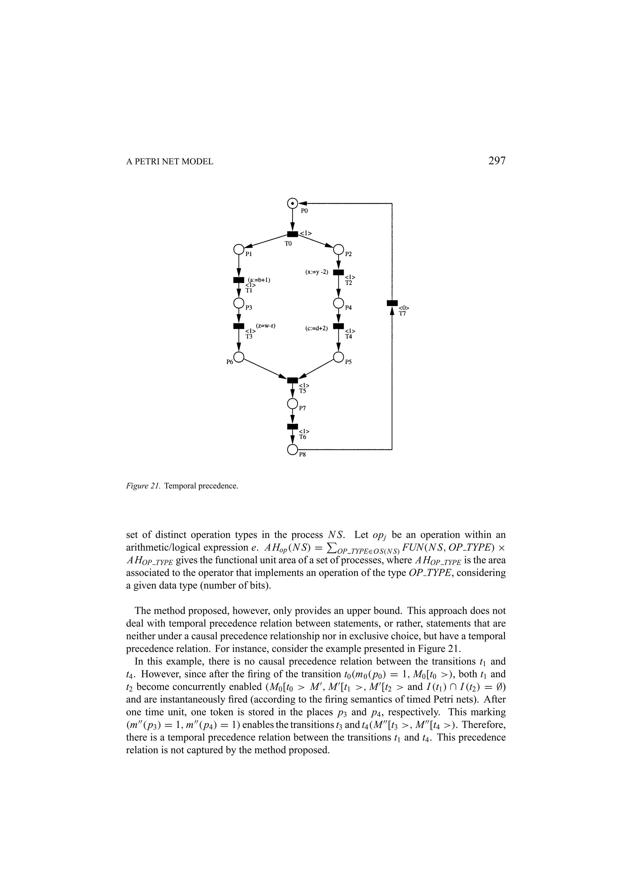
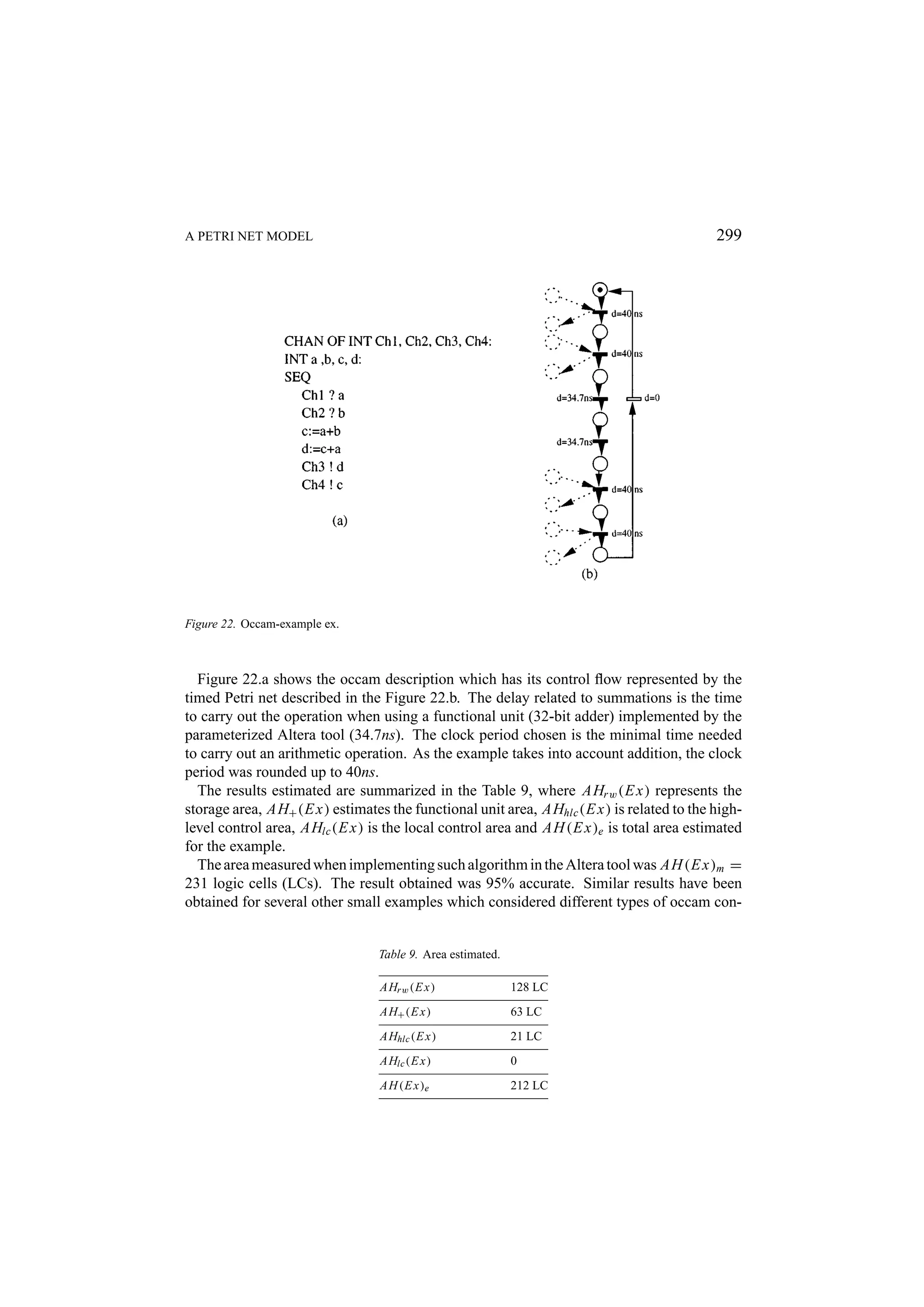
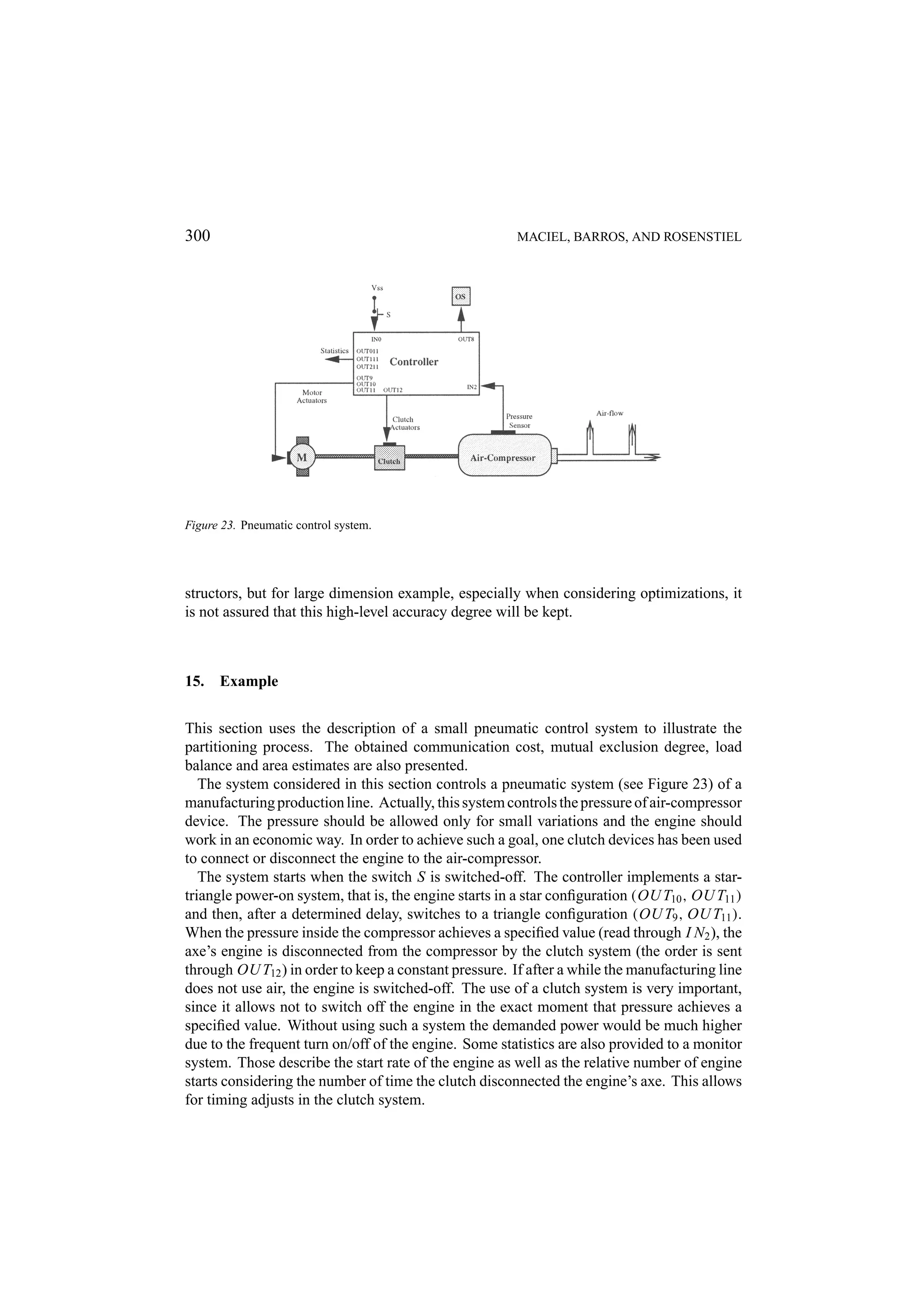
A PETRI NET MODEL 301 Figure 24. Functional diagram. The occam program representing this pneumatic control system is composed of eleven simple processes. Theses processes exchange information through channels according to CSP semantics. Figure 24 shows a block diagram representing the connection between those processes as well as the interface points from sensors and to actuators. The occam program which implements the behavior is presented in appendix. This program was obtained after the splitting phase. Due to space restriction, the description is presented in a linear format. After the classification phase and the translation into Petri net model, the qualitative analysis can be carried out. The results obtained in this phase are presented below: B SB L REV S MG SM FC 3 Y Y Y Y Y N N Y This result presents interesting properties related to this model. The system is bounded and structurally bounded, which means that for any initial marking it is still a bounded model. The model is live, reversible and safe. If a model has such properties, all of its transitions are fired at least once. The model is also a free choice system, although it is neither a marked graph nor a state machine Petri net. Nevertheless, such a system allows a controlled conflict. The allocation process is carried out by using a clustering algorithm [74], which builds a tree by considering communication costs, processor’s load balance and mutual exclusion degree between processes [69, 70, 72, 73]. The globally normalized communication cost, locally normalized load balance and the mutual exclusion degree of pairs of processes of the example are depicted in Figure 25, respectively.

302 MACIEL, BARROS, AND ROSENSTIEL Figure 25. NCC, LME, LLB of pairs of processes. The cost function C L M(N CC, L M E, L LC, the clustering tree (allocation tree) built from this cost function as well as the cost function AC = AC(N CC( pri ), Nload( pri , p K ), L M E( pri )) are depicted in Figure 26. After obtaining clusters, one process in each cluster should be chosen to be allocated in each processor of the architecture. This choice is carried out considering the minimization of the cost function AC = AC(N CC( pri ), Nload( pri , p K ), L M E( pri )). Figure 26 also presents the communication cost and the mutual exclusion degree of each process as well as the workload of each process for the Transputer T 800 and a summary of the cost function AC. Considering a target architecture with two microprocessors (Transputer T800 in this case), the allocation algorithm chooses processes P9 to be allocated in one processor and process P6 to be implemented in the other one.

A PETRI NET MODEL 303 Figure 26. Allocation.

304 MACIEL, BARROS, AND ROSENSTIEL Once one process is allocated in each software component, the clustering phase takes place. In this phase a clustering tree is built according to the algorithm described in Section 4.3.2. The clustering tree, which is depicted in Figure 27.b, is based on the distance matrix presented in Figure 27.a. The clustering process results 3 clusters, one to be implemented in hardware and two to be implemented in software: each one by using a distinct microprocessor. The allocation and clustering phases have been carried out by taking into account the results of the quantitative analysis tool. Due to the high delay when implementing processes P4 and P5 in software, they should be implemented in hardware. Process P7 has also migrated to software because of the high communication cost with the process P4 . 16. Conclusion This work presented based on Petri net for hardware/software codesign which is being used in the context of the PISH co-design system. Petri nets are a powerful family of formalism which allows for qualitative and quantitative analysis of behavioral descriptions. In this work, the use of Petri nets is related to quantitative analysis in order to compute metrics for hardware/software partitioning such as communication cost, workload of processors, mutual exclusion, area and delay. The results of this analysis is being used for initial allocation of processes as well as the clustering phase, where processes are grouped in clusters to be implemented either in hardware or in software. The use of Petri net as an intermediate format allows for a more accurate metric estimation for hardware/software partitioning process, as well as provides a format that is independent of the description language. Additionally, a qualitative analysis of the description may also be performed. In order to reduce the computational complexity when calculating the mentioned codesign metrics, techniques base on structural analysis have been proposed. The computation of those metrics have been implemented in C language and also takes into account the results obtained from structural analysis provided by INA tool. Some results are illustrated by a case study represented by a pneumatic control system. The use of Petri nets opens a wide range for improvements in the PISH hardware/software codesign system. Dynamic analysis may be performed by using results of a proﬁling as probability value associated to transitions belonging to IF/ALT combiners or external data- dependent loops. Moreover, granularity of processes can be dynamically determined, along with partitioning, by the analysis of sub-nets which fulﬁlls design constraints. These improvements can be seen as future works, which become feasible due to the use of Petri net as intermediate format.

A PETRI NET MODEL 305 Figure 27. Clustering.

306 MACIEL, BARROS, AND ROSENSTIEL Appendix

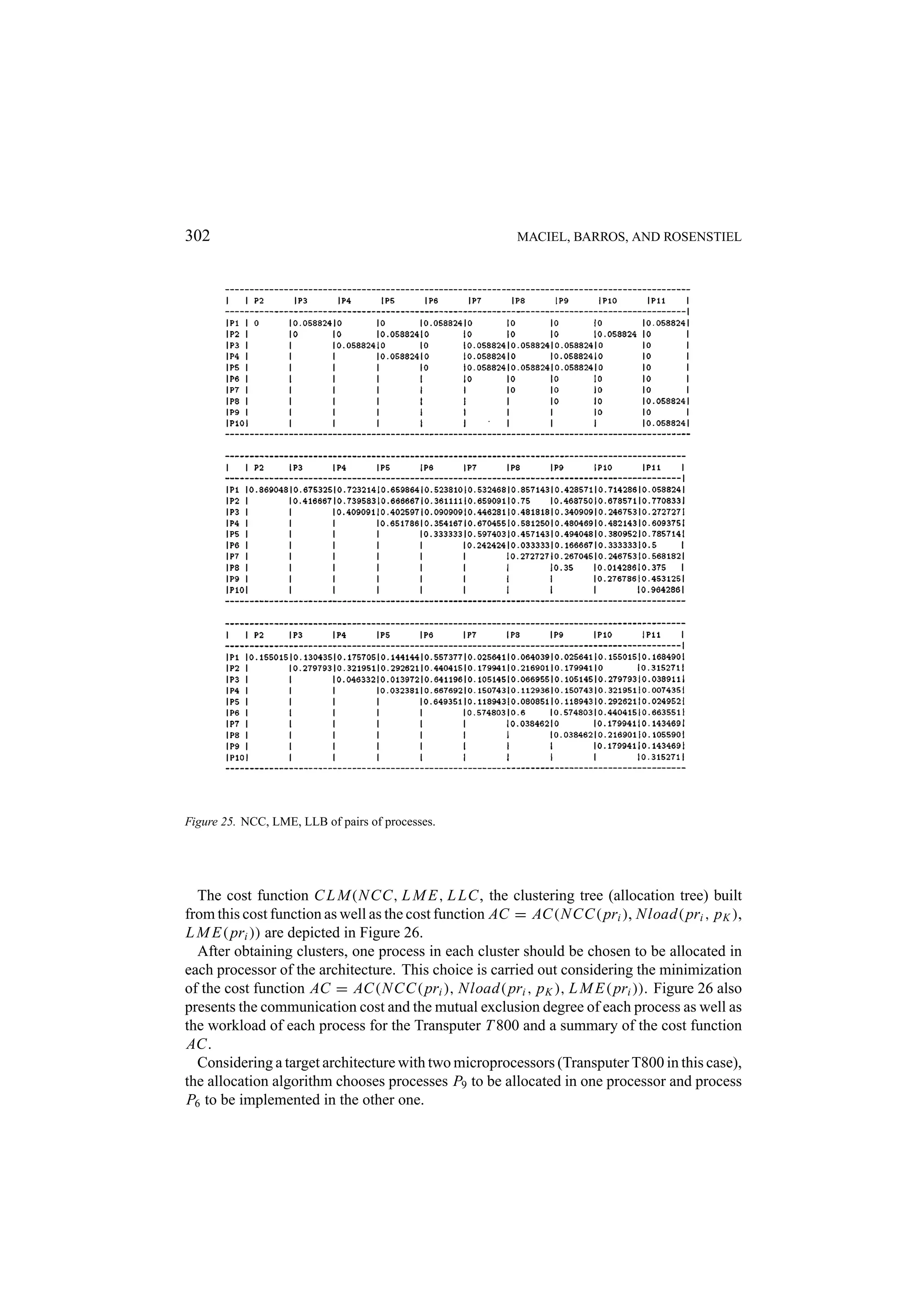
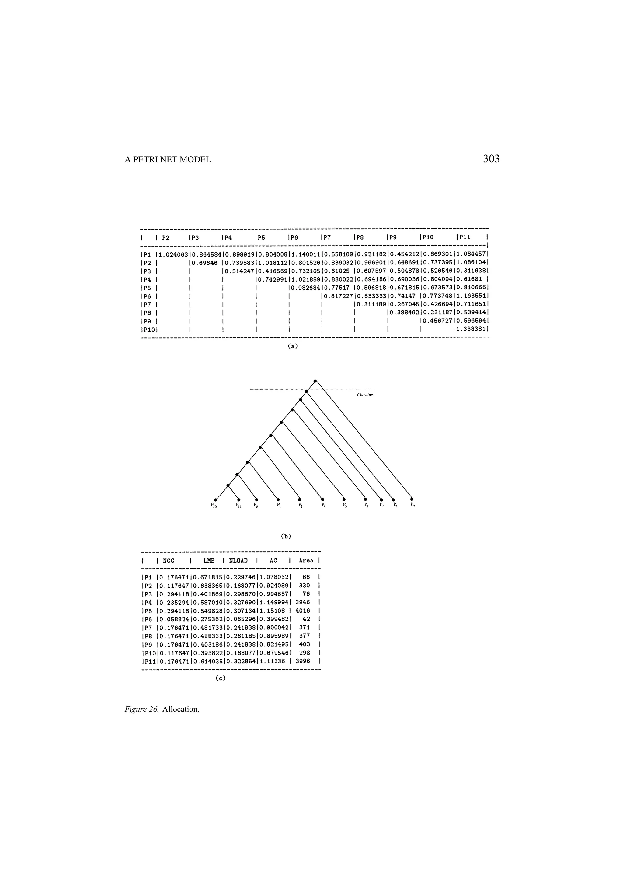
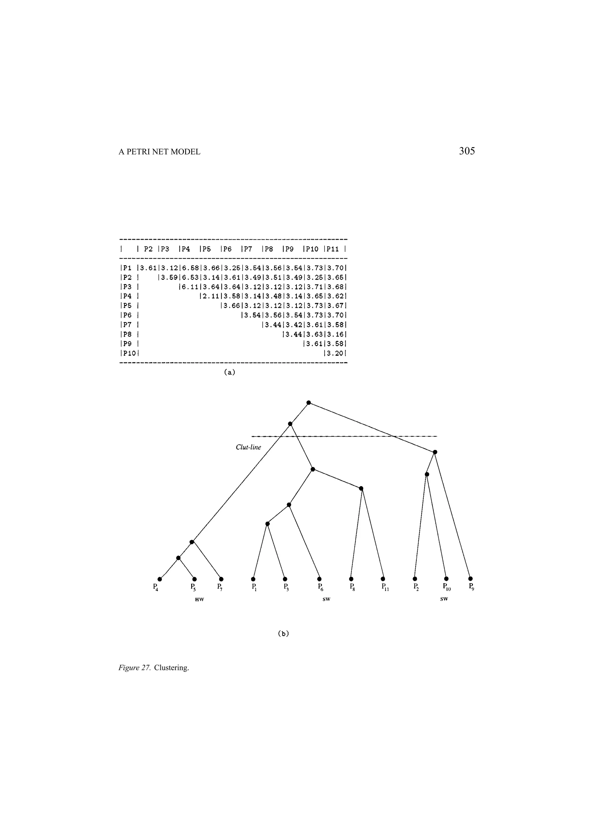
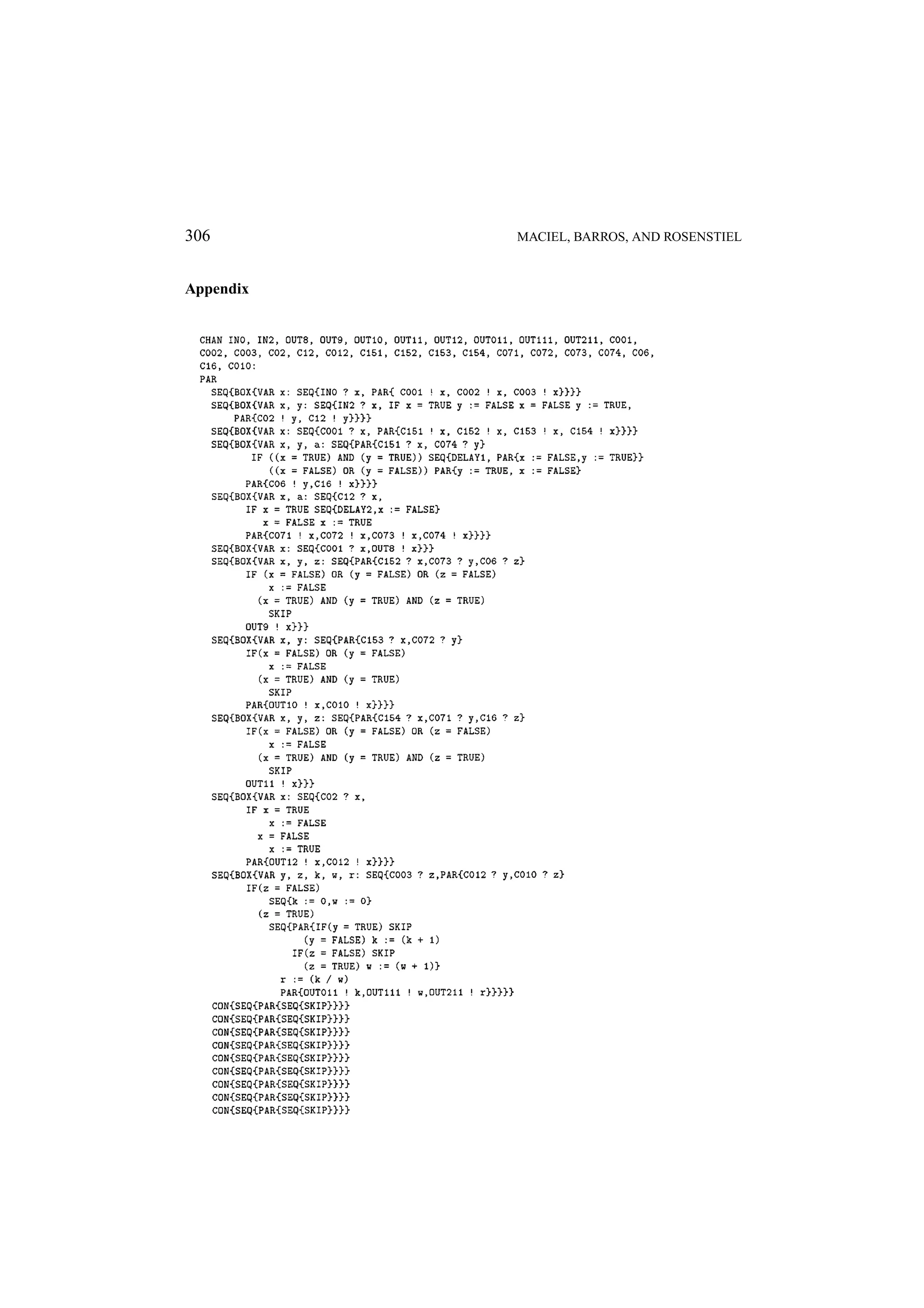
A PETRI NET MODEL 307 Acknowledgments The authors would like to thank the anonymous referees for their precise and valuable considerations. This research has been carried out with support from KIT Co-operation activity 128. Notes 1. • serial-places reduction: Let N = (R, M0 ) be a net, a transition tk , the places pi and p j . If (I (tk ) = [ pi ] and O(tk ) = [ p j ]), we may transform N = (R, M0 ) into N = (R , M0 ) by eliminating the transition tk and reducing the places pi and p j to the place pi/j such that I ( pi/j ) = I ( pi ) and O( pi/j ) = O( p j ). • parallel-places reduction: Let N = (R, M0 ) be a net, pi and p j be places and tm and tn be transitions. If I ( pi ) = I ( p j ) = [tm ] and O( pi ) = O( p j ) = [tn ], we may transform N = (R, M0 ) into N = (R , M0 ) by reducing the places pi and p j to the place pi/j such that I ( pi/j ) = I ( pi ) = I ( p j ) and O( pi/j ) = O( pi ) = O( p j ). 2. smex( pri , pr j ) represents pk ∈ pri , pr ∈ pr j M E X ( pk , pr ). r ps( pk ) and r ps( pr ) is the number of places which the places pk and pr , in the reduced net, represent in original net. 3. B-bounded, SB-structurally bounded, L-live, REV-reversible, S-safe, MG-marked graph, SM-state machine, FC-free choice. References 1. A. A. Desrochers, R. Y. Al-Jaar. Applications of Petri Nets in Manufacturing Systems. IEEE Press, 1995. 2. R. Gupta. A framework for interative analysis of timing constraints in embedded systems. Proceedings of the Fourth Codes/CASHE, pp. 44–51, IEEE Computer Society, March 1996. 3. A. Dasdan, D. Ramanathan, R. Gupta. Rate derivation and its applications to reactive, real-time embedded systems. 35th ACM Design Automation Conference, pp. 44–51, June 1998. 4. W. Wolf. Object-oriented cosynthesis of distributed embedded systems. 35th ACM Transactions on Design Automation of Electronic Systems 1(3): 301–314, July 1996. 5. S. Gaubert, J. Mairesse. Modeling and analysis of timed Petri nets using heaps of pieces LIAFA, CNRS- Universit´ Paris 7 - Report 97/14, 1997. e 6. Y. Kukimoto, R. Brayton. Exact required time analysis via false path detection. ACM Design Automation Conference, 1997. 7. F. Vahid, D. D. Gajski. Closeness metrics for systems leel functional partitioning. Proceedings of the EURO- DAC’95 pp. 328–333, IEEE Computer Society, September 1995. 8. D. D. Gajski, F. Vahid. Specification and design of embedded systems. Design and Test of Computers 53–67, Spring 1995. 9. D. D. Gajski, F. Vahid, S. Narayan, J. Gong. Specification and Design of Embedded Hardware-Software Systems. P T R Prentice Hall, 1994. 10. T. BenIsmail, M. Abid, K. O’Brien and A. Jerraya. An approach for hardware/software codesign. Proceedings of the RSP 94, Grenoble, France, 1994. 11. P. V. Knudsen and J. Madsen. PACE: A dynamic programming algorithm for hardware/software partitioning. Fourth International Workshop on HW/SW Codesign, pp. 85–92, IEEE Press, 1996. 12. C. Carreras, J. C. L´ pez, M. L. L´ pez, C. Delgado-Kloos, N. Martin´ z, and L. S´ nchez. A co-design o o e a methodology based on formal specification and high-level estimation. Fourth International Workshop on HW/SW Codesign, pp. 28–35, IEEE Press, 1996. 13. T. Cheung, G. Hellestrand and P. Kanthamanon. A multi-level transformation approach to HW/SW codesign: A case study. Fourth International Workshop on HW/SW Codesign, pp. 10–17, IEEE Press, 1996. 14. E. Barros. Hardware/Software Partitioning Using UNITY. Universit¨ t T¨ bingen, 1993. a u

308 MACIEL, BARROS, AND ROSENSTIEL 15. E. Barros and W. Rosenstiel. A clustering approach to support hardware/software partitioning. In Jerzy Rozenblit and Klaus Buchenrieder, editors, Computer Aided Software/Hardware Engineering, IEEE Press. 16. E. Barros and A. Sampaio. Towards provably correct hardware/software partitioning using occam. Pro- ceedings of the Third International Workshop on Hardware/Software Codesign Codes/CASHE94, IEEE Computer Society, September 1994. 17. E. Barros, X. Xiong and W. Rosenstiel. Hardware/software partitioning with UNITY. Handouts of Interna- tional Workshop on Hardware-Software Co-design, 1993. 18. R. Ernst and J. Henkel. Hardware-software codesign of embedded controllers based on hardware extraction. Handouts of the International Workshop on Hardware-Software Co-Design, October 1992. 19. R. Ernst and J. Henkel. A path-based technique for estimating hardware runtime in HW/SW-cosynthesis. IEEE/ACM Proc. of 8th Int’l Symp. on System Level Synthesis, October 1995. 20. R. Gupta and G. De Micheli. System-level synthesis using re-programmable components. Microprogram- ming and Microprocessing 27: 239–244, 1989. 21. C. Carreras, J. C. L´ pez, M. L. L´ pez, C. Delgado-Kloos, N. Martńez, L. S´ nchez. A co-design methodology o o ı a based on formal specification and high level estimation. Proceedings of EDAC, pp. 2–7, 1996. 22. F. Rose, T. Carpenter, S. Kumar, J. Shackleton, T. Steeves. A model for the coanalysis of hardware and software architecture. Proceedings of the Fourth Codes/CASHE, pp. 94–103, IEEE Computer Society, March 1996. 23. R. Gupta, G. De Micheli. Constrained software generation for hardware-software systems. Proceedings of the Fourth Codes/CASHE, pp. 56–63, IEEE Computer Society. September 1995. 24. P. Eles, K. Kuchcinki, Z. Peng, M. Minea. Synthesis of VHDL concurrent processes. Proceedings of the EURO-DAC’94, pp. 540–545, IEEE Computer Society, September 1994. 25. X. Gu, K. Kuchcinki, Z. Peng. Testability analysis and improvement from VHDL behavioural specification. Proceedings of the EURO-DAC’94, pp. 644–649, IEEE Computer Society, September 1994. 26. G. W. Brams. R´ seaux de Petri: Th´ orie et Pratique, tome 1. Masson Editions, 1983. e e 27. G. W. Brams. R´ seaux de Petri: Th´ orie et Pratique, tome 2. Masson Editions, 1983. e e 28. J. L. Peterson. Petri Nets an Introduction. Prentice-Hall, Inc, 1981. 29. W. Reisig. Petri Nets: An Introduction. Springer-Verlag, 1982. 30. T. Murata. State equation, controllability, and maximal of Petri nets. IEEE Trans. on Automatic Control, 1977. 31. T. Murata. Modelling and Analysis of Concurrent Systems, Handbook of Software Engineering. Van Norstrand Reinhold Company Inc., 1984. 32. O. Botti, F. Cindio. From basic to timed net models of occam: An application to program placement. PNPM, pp. 216–221, 1991. 33. M. Silva, E. Teruel. Petri nets for the design and operation of manufacturing systems. CIMAT’96, 1996. 34. M. Silva, E. Teruel. Analysis of autonomous Petri nets with a bulk services and arrivals. 11th International Conference on Analysis and Optimization of Systems. Discrete Event Systems, Vol. 199 of Lecture Notes in Control and Information Science, pp. 131–143, 1994. 35. A. Valmari. Stubborn sets for reduced state space generation. Advanced in Petri Nets. In G. Rozenberg, editor, Lecture Notes in Computer Science 483: 491–515, Springer Verlag, 1991. 36. A. Valmari. Compositional state space generation. Advanced in Petri Nets. In G. Rozenberg, editor, Lecture Notes in Computer Science 674: 427–457, Springer Verlag, 1993. 37. T. Murata. Petri nets: Properties, analysis and applications. Proceeding of the IEEE, 1989. 38. G. Berthelot. Checking properties of nets using transformations. Advanced in Petri Nets. In G. Rozenberg, editor, Lecture Notes in Computer Science 222: 19–40, Springer Verlag, 1986. 39. K. Jensen. Coloured Petri nets: Basic concepts, analysis methods and practical uses. EACTS Monographs on Theoretical Computer Science. Springer Verlag, 1994. 40. I. Gorton. Parallel program design using high-level Petri nets. Concurrency: Practice and Experience, 1993. 41. G. Dohmen. Petri nets as intermediate representation between VHDL and symbolic transition systems. Proceedings EURODAC-94, 1994. 42. J. Esparza, M. Nielsen. Decidability issues for Petri nets. Gesellschaft f¨ r Informatik, 1994. u 43. C. Rackoff. The covering and boundedness problem for vector addition systems. Theoretical Computer Science 6: 223–231, 1978. 44. R. Karp, R. Miller. Parallel program schemata. Journal of Computer and System Science 3(4): 167–195, 1969.

A PETRI NET MODEL 309 45. R. Lipton. The reachability problem requires exponential space. Research Report 62, Department of Com- puter Science, Yale University, 1976. 46. G. S. Sacerdote, R. L. Tenney. The decidibility of the reachability problem for vector addition system. 9th Annual Symposium on Theory of Computing, 61–76. 47. E. W. Mayr. Persistence of vector replacement system is decidable. Acta Informatica 15: 309–318, 1981. Boulder, 1977. 48. S. R. Kosaraju. Decidibility of reachability in vector addition systems. 14th Annual ACM Symposium on Theory of Computing, San Francisco, 1982, pp. 267–281. 49. J. L. Lambert. Vector addition systems and semi-linearity. SIAM Journal of Computing, 1994. 50. D. Frutos, C. Johne. Decidability of home states in place transition systems. 14th Internal Report, Dpto. Informatica y Automatica, Univ. Complutense de Madrid, 1986. 51. E. Cardoza, R. J. Lipton, A. R. Meyer. Exponential space complete problems for Petri nets and commutative semigroups. 8th Symposium on Theory of Computing, 50–54, 1976. 52. M. H. T. Hack. Decidability Questions for Petri Nets. PhD Thesis, MIT, 1976. 53. A. Cheng, J. Esparza, J. Palsberg. Complexity results for 1-safe nets. 13th Conference on Foundations of Software Technology and Theoretical Computer Science, Bombay, 1993. 54. J. Grabowsky. The decidability of persistence for vector addition systems. Information Processing Letters 11 1: 20–23, 1980. 76.block Boulder, 1977. 55. H. M¨ ller. On the reachability problem for persistent vector replacement systems. Computing Supplements u 3: 89–104, 1981. 56. K. Jensen. Coloured Petri nets: A high level language for system design and analysis. Lecture Notes in Computer Science 483: 342–416, 1990. 57. Ramchandani. Analysis of asynchronous concurrent systems by timed Petri nets. Technical Report n 120 , Laboratory for Computer Science, MIT, Cambridge, MA, 1974. 58. K. Jensen, P. Huber, R. M. Shapiro. Hierarchies in coloured Petri nets. In G. Rozenberg, editor, Lecture Notes in Computer Science 483: 313–341, Springer-Verlag, 1990. 59. P. R. M. Maciel, E. N. S. Barros. Captura de requisitos temporais usando redes de Petri para o particionamento c˜ de hardware/software. IX Simp´ sio Brasileiro de Concep¸ ao de Circuitos Integrados, Recife, PE, 1996, o pp. 383–396. 60. C. A. R. Hoare. Communicating Sequential Processes. Prentice Hall International, 1985. 61. P. R. M. Maciel, E. N. S. Barros. Capturing time constraints by using Petri nets in the context of hardware/software codesign. a ser publicado no 7th IEEE International Workshop on Rapid System Prototyping, Porto Caras, Thessaloniki, Gr´ cia, 1996. e 62. G. Jones. Programming in OCCAM. C. A. R. Hoare Series Editor, Prentice-Hall International Series in Computer Science, 1987. 63. L. Silva, A. Sampaio and E. Barros. A normal form reduction strategy for hardware/software partitioning. Conference Formal Methods Europe’97, 1997. c˜ ` c˜ 64. P. R. M. Maciel, R. D. Lins, P. R. F. Cunha. Uma Introdu¸ ao as Redes de Petri e Aplica¸ oes. Book published in the 11th Escola de Computa¸ ao. Campinas, Brazil. July, 1996. (portuguese) c˜ 65. W. W. Chu, L. J. Holloway, M. T. Lang, K. Efe. Task allocation in distributed data processing. IEEE-Computer 57–68, November 1980. 66. V. M. Lo. Heuristic algorithms for task assignment is distributed systems. IEEE Transactions on Computers 37(11): 1384–1397, November 1988. 67. C. E. Houstis. Module allocation of real-time applications to distributed systems. IEEE Transactions on Software Engineering 5(7): 699–709, July 1990. 68. W. W. Chu, L. M-T. Lan. Task allocation and precedence relations for distributed real-time systems. IEEE Transactions on Computers C-36(6): 667–679, June 1987. 69. P. Maciel, E. Barros, W. Rosenstiel. Computing communication cost by Petri nets for hardware/software codesign. 8th IEEE International Workshop on Rapid System Prototyping, Chapel Hill, North Carolina, June 24–26, 1997. 70. P. Maciel, E. Barros, W. Rosenstiel. Using Petri nets to compute communication cost for hardware/software codesign. Published on the 10th Brazilian Symposium on Integrated Circuit Design, Gramado, Rio Grande do Sul, Brazil, August 25–27, 1997. 71. P. M. Merlin, D. J. Farber. Recoverability of communication protocols implications of a theoretical study. IEEE Transaction Communication COM-24, September 1976. 72. P. Maciel, T. Maciel, E. Barros, W. Rosenstiel. A Petri net approach to compute load balance in hardware/software codesign. High Performance Computing ’98, Boston, Massachusetts, April 5–9, 1998.

310 MACIEL, BARROS, AND ROSENSTIEL 73. P. Maciel, E. Barros, W. Rosenstiel. A Petri net approach for quantifying mutual exclusion degree. IN- COM’98, Nancy-Metz, France, June 23–27, 1998. 74. P. Maciel, E. Barros, W. Rosenstiel. A Petri net based approach for performing the initial allocation in hardware/software codesign. 1998 IEEE International Conference on Systems, Man, and Cybernetics, San Diego, October 11–14, 1998. 75. P. Maciel, E. Barros, W. Rosenstiel. A Petri net approach to compute load balance in hardware/software codesign. To be published on the High Performance Computing ’99, San Diego, April 1999. 76. N. G. Leveson, J. L. Stolzy. Safety analysis using Petri nets. IEEE Transaction Software Eng. SE-13(3): March 1987. 77. W. M. Zubarek. Timed Petri nets definitions, properties and applications. Microelectronic and Reliability 31(4): 627–644, 1991. 78. P. H. Starke. Remarks on timed Petri nets. Proc. 9th European Workshop on Application and Theory of Petri Nets, 1988. 79. M. Ajmone-Marsan. Stochastic Petri nets: An elementary introduction. LNCS vol. 424, Springer Verlag, 1989. 80. M. K. Molloy. On the Integration of Delay and Throughput Measures in Distributed Processing Models. Ph.D. Thesis, UCLA, Los Angeles, CA, 1981. 81. S. Gaubert. Performance evaluation of (max, +) automata. IEEE Transaction on Automatic Control, 1995. 82. C. Ghezzi, D. Mandrioli, S. Morasca, M. Pezz. A unified high-level Petri net formalism for time-critical systems. IEEE Transactions on Software Engineering, February 1991. 83. J. Sifakis. Use of Petri nets for performance evaluation. Measuring, Modelling and Evaluating Computer Systems, North Holland, 1977. 84. J. M. Colom, M. Silva. Convex geometry and semiflows in P/T nets. A comparative study of algorithms for computation of minimal P-semiflows. In G. Rozenberg, editor, Lecture Notes in Computer Science 483: 79–112, Springer-Verlag, 1990. 85. F. Bowden. Modeling time in Petri nets. 2th Australia-Japan Workshop on Stochastic Models, Gold Coast, July 1996. 86. J. M. Colom, M. Silva. Improving the linearly based characterization of P/T nets. In G. Rozenberg, editor, Lecture Notes in Computer Science 483: 113–145, Springer-Verlag, 1990. 87. F. Dicesare, G. Harhalakis, J. M. Proth, M. Silva, F. B. Vernadat. Practice of Petri Nets in Manufacturing. Chapman and Hall, 1993. 88. M. Zhou, F. Dicesare. Petri Net Synthesis for Discrete Event Control of Manufacturing Systems. Kluwer Academic Publishers, 1993. 89. C. Lindemann. Performance Modelling with Deterministic and Stochastic Petri Nets. John Wiley and Sons, 1998. 90. S. Malik, M. Martonosi, Yau-Tsun L. Static timing analysis of embedded software. Design Automation Conference, 1997. 91. F. Ercal, J. Ramanuajam, P. Sadayappan. Task allocation onto a hypercube by recursive minicut bipartition- ing. Journal of Parallel and Distributed Computing 10: 35–44, 1990. 92. C. Cohen, S. Gaubert, J. Quadrat. Algebraic system analysis of timed Petri nets. In J. Gunawardena, editor, Idempotency - Collection of Isaac Newton Institute, Cambridge University Press, 1995. 93. R. Spencer and A. Sampaio. De occam para o Transputer: Compila¸ ao via Reescrita de Termos. Anais do c˜ X Simp´ sio Brasileiro de Engenharia de Software, S˜ o Carlos-SP, 1996, pp. 103–117. o a 94. M. E. de Lima and D. J. Kinniment. Hierarchial placement method based on a force-directed algorithm and simultaneous global routing for sea-of-gates. IEE Proceedings, Computing. Digit. Tech. 143(1): 1–8, January 1996. 95. K. A. Bartlett, R. K. Brayton, G. D. Hachtel, R. M. Jacoby, C. R. Morrison, R. L. Rudell, A. Vicentelli, A. Wang. Multilevel logic minimization using implicit don’t cares. IEEE Transactions on CAD 7(6), June 1988. 96. R. Camposano, W. Rosenstiel. Synthesizing circuits from behavioral descriptions. IEEE Transactions on CAD of Integrated Circuits and Systems 8(2): 171–180, February 1989. 97. G. Borriello. Combining event and data flow graphs in behavioral synthesis. Proceeding of the ICCAD, pp. 56–59, 1988. 98. D. De Micheli, D. Ku, F. Mailhot and T. Trunong. The Olympus Synthesis System. IEEE Design and Test of Computers, October 1990.

A petri net model for hardware software codesign

More Related Content

What's hot

Viewers also liked

Similar to A petri net model for hardware software codesign

More from JULIO GONZALEZ SANZ

A petri net model for hardware software codesign