
| |  在 GitHub 中查看源代码 在 GitHub 中查看源代码 |
概述
使用 TensorFlow Image Summary API,您可以轻松地在 TensorBoard 中记录张量和任意图像并进行查看。这在采样和检查输入数据,或可视化层权重和生成的张量方面非常实用。您还可以将诊断数据记录为图像,这在模型开发过程中可能会有所帮助。
在本教程中,您将了解如何使用 Image Summary API 将张量可视化为图像。您还将了解如何获取任意图像,将其转换为张量并在 TensorBoard 中进行可视化。教程将通过一个简单而真实的示例,向您展示使用图像摘要了解模型性能。
设置
下载 Fashion-MNIST 数据集
您将构造一个简单的神经网络,用于对 Fashion-MNIST 数据集中的图像进行分类。此数据集包含 70,000 个 28x28 灰度时装产品图像,来自 10 个类别,每个类别 7,000 个图像。
首先,下载数据:
# Download the data. The data is already divided into train and test. # The labels are integers representing classes. fashion_mnist = keras.datasets.fashion_mnist (train_images, train_labels), (test_images, test_labels) = \ fashion_mnist.load_data() # Names of the integer classes, i.e., 0 -> T-short/top, 1 -> Trouser, etc. class_names = ['T-shirt/top', 'Trouser', 'Pullover', 'Dress', 'Coat', 'Sandal', 'Shirt', 'Sneaker', 'Bag', 'Ankle boot'] Downloading data from https://storage.googleapis.com/tensorflow/tf-keras-datasets/train-labels-idx1-ubyte.gz 32768/29515 [=================================] - 0s 0us/step Downloading data from https://storage.googleapis.com/tensorflow/tf-keras-datasets/train-images-idx3-ubyte.gz 26427392/26421880 [==============================] - 0s 0us/step Downloading data from https://storage.googleapis.com/tensorflow/tf-keras-datasets/t10k-labels-idx1-ubyte.gz 8192/5148 [===============================================] - 0s 0us/step Downloading data from https://storage.googleapis.com/tensorflow/tf-keras-datasets/t10k-images-idx3-ubyte.gz 4423680/4422102 [==============================] - 0s 0us/step
可视化单个图像
为了解 Image Summary API 的工作原理,现在您将在 TensorBoard 中记录训练集中的第一个训练图像。
在此之前,请检查训练数据的形状:
print("Shape: ", train_images[0].shape) print("Label: ", train_labels[0], "->", class_names[train_labels[0]]) Shape: (28, 28) Label: 9 -> Ankle boot
请注意,数据集中每个图像的形状均为 2 秩张量,形状为 (28, 28),分别表示高度和宽度。
但是,tf.summary.image() 需要一个包含 (batch_size, height, width, channels) 的 4 秩张量。因此,需要重塑张量。
您仅记录一个图像,因此 batch_size 为 1。图像为灰度图,因此将 channels 设置为 1。
# Reshape the image for the Summary API. img = np.reshape(train_images[0], (-1, 28, 28, 1)) 现在,您可以在 TensorBoard 中记录此图像并进行查看了。
# Clear out any prior log data. !rm -rf logs # Sets up a timestamped log directory. logdir = "logs/train_data/" + datetime.now().strftime("%Y%m%d-%H%M%S") # Creates a file writer for the log directory. file_writer = tf.summary.create_file_writer(logdir) # Using the file writer, log the reshaped image. with file_writer.as_default(): tf.summary.image("Training data", img, step=0) 现在,使用 TensorBoard 检查图像。等待几秒,直至界面出现。
%tensorboard --logdir logs/train_data 
“Time Series”信息中心显示您刚刚记录的图像。这是一只“短靴”。
图像会缩放到默认大小,以方便查看。如果要查看未缩放的原始图像,请选中右侧“Settings”面板底部的“Show actual image size”。
调整亮度和对比度滑块,查看它们如何影响图像像素。
可视化多个图像
记录一个张量非常简单,但是要记录多个训练样本应如何操作?
只需在向 tf.summary.image() 传递数据时指定要记录的图像数即可。
with file_writer.as_default(): # Don't forget to reshape. images = np.reshape(train_images[0:25], (-1, 28, 28, 1)) tf.summary.image("25 training data examples", images, max_outputs=25, step=0) %tensorboard --logdir logs/train_data 
记录任意图像数据
如果要可视化的图像并非张量(例如 matplotlib 生成的图像),应如何操作?
您需要一些样板代码来将图转换为张量,随后便可继续处理。
在以下代码中,您将使用 matplotlib 的 subplot() 函数以美观的网格结构记录前 25 个图像。随后,您将在 TensorBoard 中查看该网格:
# Clear out prior logging data. !rm -rf logs/plots logdir = "logs/plots/" + datetime.now().strftime("%Y%m%d-%H%M%S") file_writer = tf.summary.create_file_writer(logdir) def plot_to_image(figure): """Converts the matplotlib plot specified by 'figure' to a PNG image and returns it. The supplied figure is closed and inaccessible after this call.""" # Save the plot to a PNG in memory. buf = io.BytesIO() plt.savefig(buf, format='png') # Closing the figure prevents it from being displayed directly inside # the notebook. plt.close(figure) buf.seek(0) # Convert PNG buffer to TF image image = tf.image.decode_png(buf.getvalue(), channels=4) # Add the batch dimension image = tf.expand_dims(image, 0) return image def image_grid(): """Return a 5x5 grid of the MNIST images as a matplotlib figure.""" # Create a figure to contain the plot. figure = plt.figure(figsize=(10,10)) for i in range(25): # Start next subplot. plt.subplot(5, 5, i + 1, title=class_names[train_labels[i]]) plt.xticks([]) plt.yticks([]) plt.grid(False) plt.imshow(train_images[i], cmap=plt.cm.binary) return figure # Prepare the plot figure = image_grid() # Convert to image and log with file_writer.as_default(): tf.summary.image("Training data", plot_to_image(figure), step=0) %tensorboard --logdir logs/plots 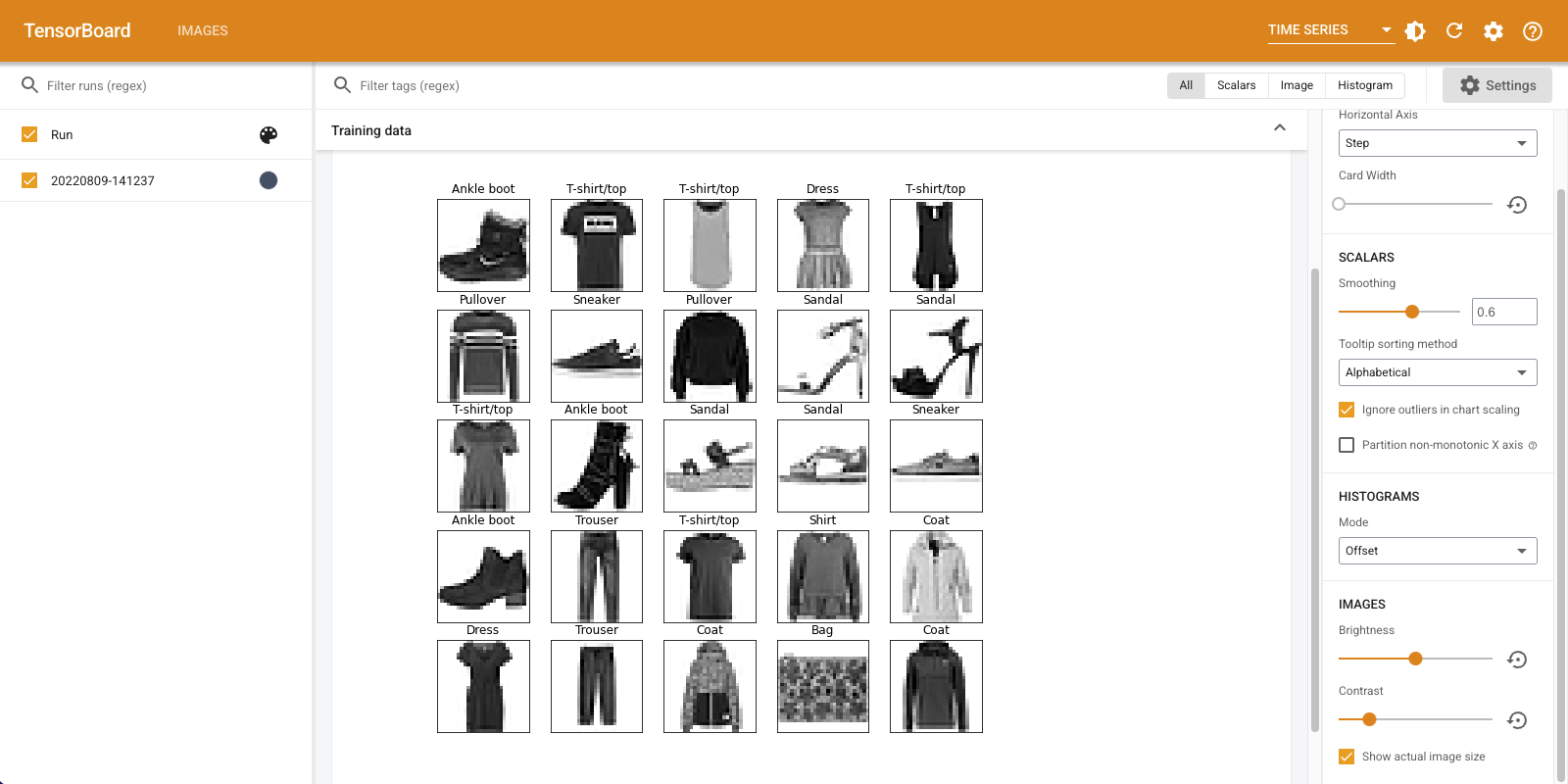
构建图像分类器
现在,让我们将其运用于实例当中。毕竟,我们是在研究机器学习,而不是绘制漂亮的图片!
您将使用图像摘要来了解模型性能,同时为 Fashion-MNIST 数据集训练一个简单的分类器。
首先,创建一个非常简单的模型并通过设置优化器和损失函数对该模型进行编译。在编译步骤中,还需指定您要定期记录其准确率的分类器。
model = keras.models.Sequential([ keras.layers.Flatten(input_shape=(28, 28)), keras.layers.Dense(32, activation='relu'), keras.layers.Dense(10, activation='softmax') ]) model.compile( optimizer='adam', loss='sparse_categorical_crossentropy', metrics=['accuracy'] ) 训练分类器时,查看混淆矩阵非常实用。混淆矩阵可帮助您详细了解分类器在测试数据上的性能。
定义一个计算混淆矩阵的函数。您将使用便捷的 Scikit-learn 函数进行定义,然后使用 matplotlib 绘制混淆矩阵。
def plot_confusion_matrix(cm, class_names): """ Returns a matplotlib figure containing the plotted confusion matrix. Args: cm (array, shape = [n, n]): a confusion matrix of integer classes class_names (array, shape = [n]): String names of the integer classes """ figure = plt.figure(figsize=(8, 8)) plt.imshow(cm, interpolation='nearest', cmap=plt.cm.Blues) plt.title("Confusion matrix") plt.colorbar() tick_marks = np.arange(len(class_names)) plt.xticks(tick_marks, class_names, rotation=45) plt.yticks(tick_marks, class_names) # Compute the labels from the normalized confusion matrix. labels = np.around(cm.astype('float') / cm.sum(axis=1)[:, np.newaxis], decimals=2) # Use white text if squares are dark; otherwise black. threshold = cm.max() / 2. for i, j in itertools.product(range(cm.shape[0]), range(cm.shape[1])): color = "white" if cm[i, j] > threshold else "black" plt.text(j, i, labels[i, j], horizontalalignment="center", color=color) plt.tight_layout() plt.ylabel('True label') plt.xlabel('Predicted label') return figure 现在,您可以训练分类器并定期记录混淆矩阵了。
您将执行以下操作:
- 创建 Keras TensorBoard 回调以记录基本指标
- 创建 Keras LambdaCallback 以在每个周期结束时记录混淆矩阵
- 使用 Model.fit() 训练模型,确保传递两个回调
随着训练的进行,向下滚动以查看 TensorBoard 启动情况。
# Clear out prior logging data. !rm -rf logs/image logdir = "logs/image/" + datetime.now().strftime("%Y%m%d-%H%M%S") # Define the basic TensorBoard callback. tensorboard_callback = keras.callbacks.TensorBoard(log_dir=logdir) file_writer_cm = tf.summary.create_file_writer(logdir + '/cm') def log_confusion_matrix(epoch, logs): # Use the model to predict the values from the validation dataset. test_pred_raw = model.predict(test_images) test_pred = np.argmax(test_pred_raw, axis=1) # Calculate the confusion matrix. cm = sklearn.metrics.confusion_matrix(test_labels, test_pred) # Log the confusion matrix as an image summary. figure = plot_confusion_matrix(cm, class_names=class_names) cm_image = plot_to_image(figure) # Log the confusion matrix as an image summary. with file_writer_cm.as_default(): tf.summary.image("epoch_confusion_matrix", cm_image, step=epoch) # Define the per-epoch callback. cm_callback = keras.callbacks.LambdaCallback(on_epoch_end=log_confusion_matrix) # Start TensorBoard. %tensorboard --logdir logs/image # Train the classifier. model.fit( train_images, train_labels, epochs=5, verbose=0, # Suppress chatty output callbacks=[tensorboard_callback, cm_callback], validation_data=(test_images, test_labels), ) 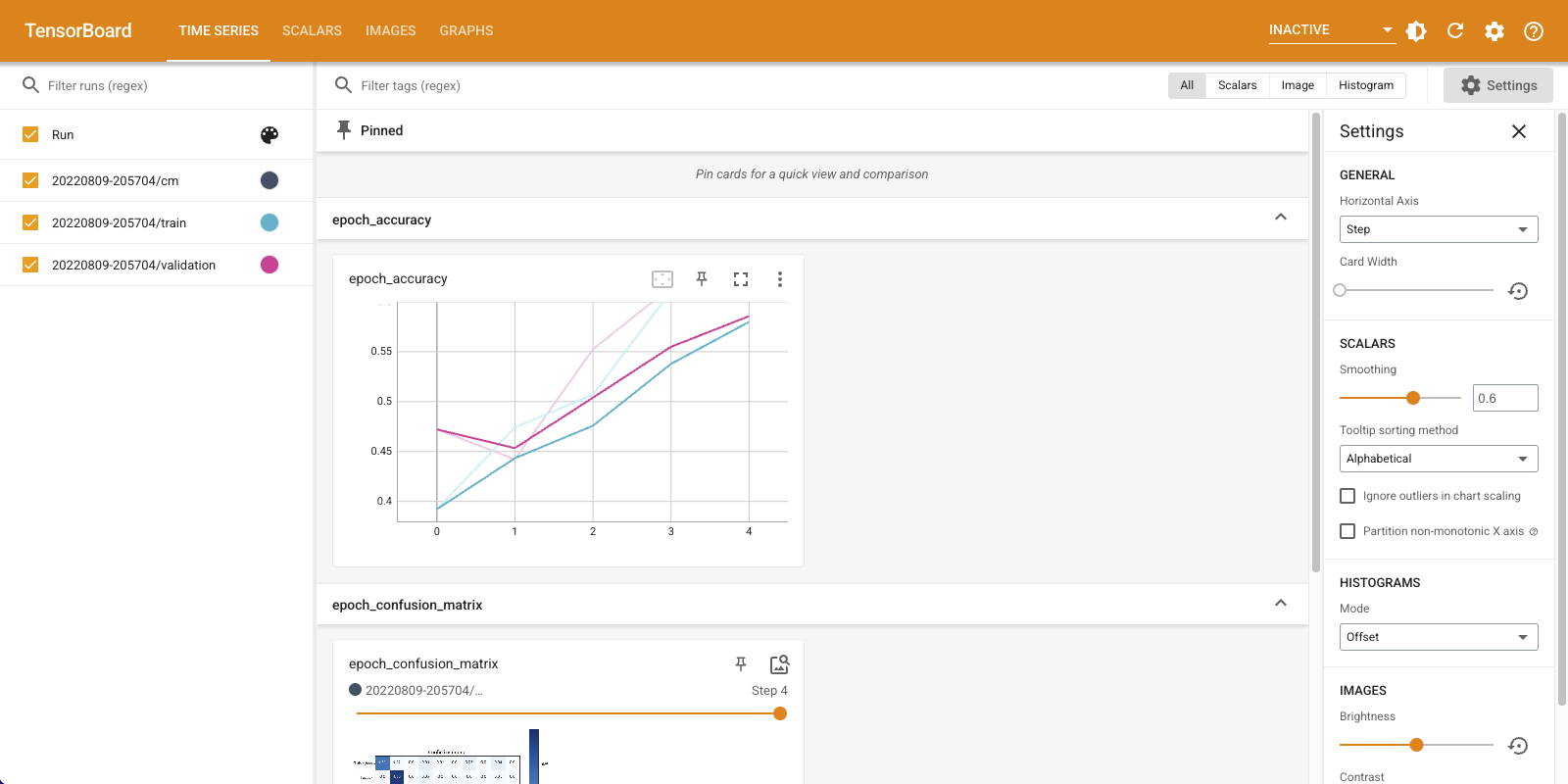
请注意,模型在训练集和验证集上的准确率都在提高。这是一个好迹象。但是,该模型在数据特定子集上的性能如何呢?
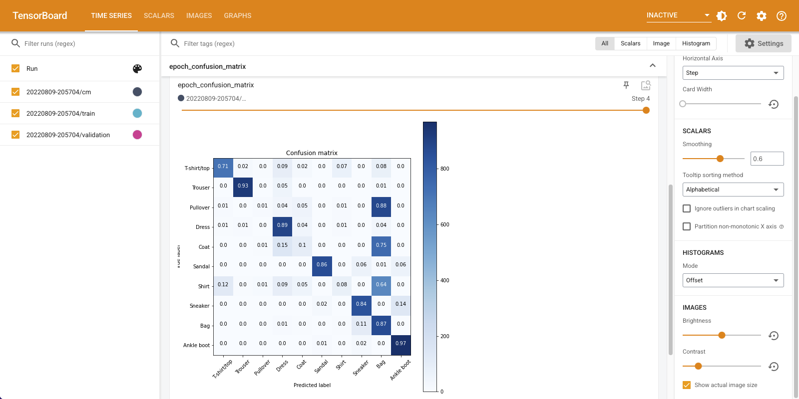
向下滚动“Time Series”信息中心以呈现记录的混淆矩阵。选中“Settings”面板底部的“Show actual image size”以查看全尺寸的混淆矩阵。
默认情况下,信息中心会显示上次记录的步骤或周期的图像摘要。可以使用滑块查看更早的混淆矩阵。请注意矩阵随训练进行而发生的显著变化:深色的正方形会沿对角线聚集,而矩阵的其余部分则趋于 0 和白色。这意味着您的分类器的性能会随着训练的进行而不断提高!做得好!
混淆矩阵表明此简单模型存在一些问题。尽管已取得重大进展,但在衬衫、T 恤和套头衫之间却出现混淆。该模型需要进一步完善。
如果您有兴趣,请尝试使用卷积神经网络 (CNN) 改进此模型。