Data Visualization
A picture is worth a thousand words. In machine learning, we usually handle high-dimensional data, which is impossible to draw on display directly. But a variety of statistical plots are tremendously valuable for us to grasp the characteristics of many data points. Smile provides data visualization tools such as plots and maps for researchers to understand information more easily and quickly.
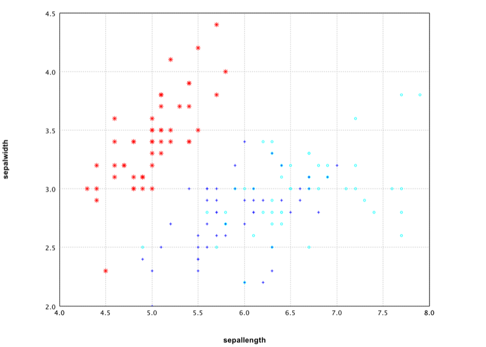
Scatter Plot
A scatter plot displays data as a collection of points. The points can be color-coded, which is very useful for classification tasks. The user can use plot functions to draw scatter plot easily.
def plot(x: Array[Array[Double]], mark: Char = '*', color: Color = Color.BLACK): Canvas def plot(x: Array[Array[Double]], y: Array[String], mark: Char): Canvas def plot(x: Array[Array[Double]], y: Array[Int], mark: Char): Canvas public class ScatterPlot { public static ScatterPlot of(double[][] points, char mark, Color color); public static ScatterPlot of(double[][] x, String[] y, char mark); public static ScatterPlot of(double[][] x, int[] y, char mark); } The legends are as follows.
-
.: dot -
+: + -
-: - -
|: | -
*: star -
x: x -
o: circle -
O: large circle -
@: solid circle -
#: large solid circle -
s: square -
S: large square -
q: solid square -
Q: large solid square
For any other char, the data point will be drawn as a dot.
The functions return a Canvas, which can be used to control the plot programmatically. The user can also use the popup context menu by right mouse click to print, change the title, axis labels, and font, etc. To display the canvas on desktop, call show(canvas), which will render the plot properly with an implicit renderer engine.
For both 2D and 3D plot, the user can zoom in/out by mouse wheel. For 2D plot, the user can shift the coordinates by moving mouse after double click. The user can also select an area by mouse for detailed view. For 3D plot, the user can rotate the view by dragging mouse.
val iris = read.arff("data/weka/iris.arff") val canvas = plot(iris, "sepallength", "sepalwidth", "class", '*') canvas.figure.setAxisLabels("sepallength", "sepalwidth") show(canvas) import java.awt.Color; import smile.io.*; import smile.plot.swing.*; import smile.plot.swing.Histogram; import smile.stat.distribution.*; import smile.math.matrix.*; import smile.util.function.*; import smile.interpolation.BicubicInterpolation; var iris = Read.arff("data/weka/iris.arff"); var figure = ScatterPlot.of(iris, "sepallength", "sepalwidth", "class", '*').figure(); figure.setAxisLabels("sepallength", "sepalwidth"); var pane = new FigurePane(figure); pane.window(); In this example, we plot the first two columns of Iris data. We use the class label for legend and color coding.
It is also easy to draw a 3D plot.
val canvas = plot(iris, "sepallength", "sepalwidth", "petallength", "class", '*') canvas.figure.setAxisLabels("sepallength", "sepalwidth", "petallength") show(canvas) var figure = ScatterPlot.of(iris, "sepallength", "sepalwidth", "petallength", "class", '*').figure(); figure.setAxisLabels("sepallength", "sepalwidth", "petallength"); var pane = new FigurePane(figure); pane.window(); 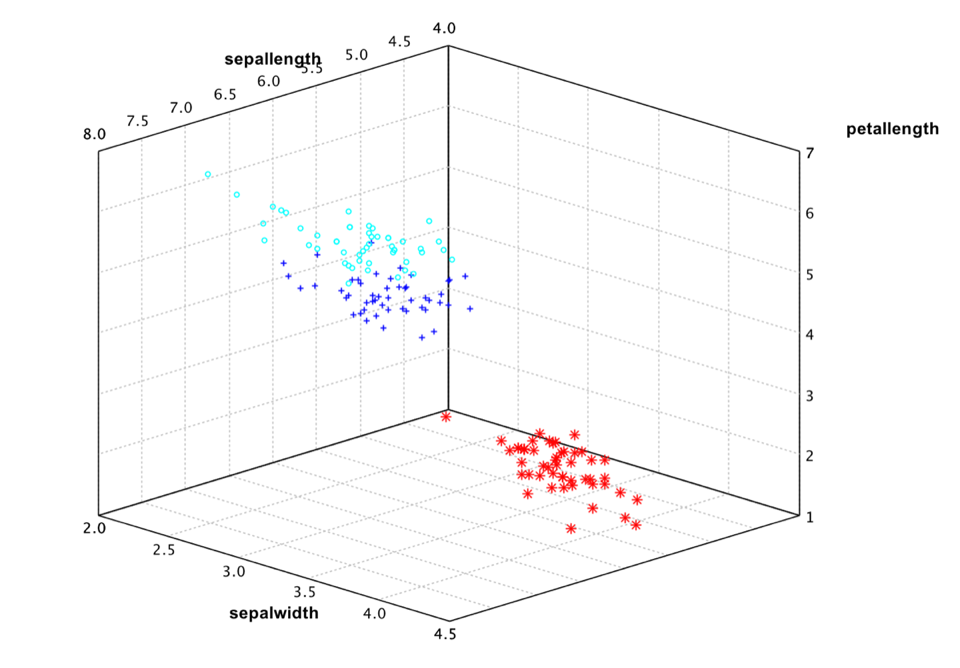
However, the Iris data has four attributes. So even 3D plot is not sufficient to see the whole picture. A general practice is plot all the attribute pairs. For example,
show(splom(iris, '*', "class")) var pane = MultiFigurePane.splom(iris, '*', "class"); pane.window(); 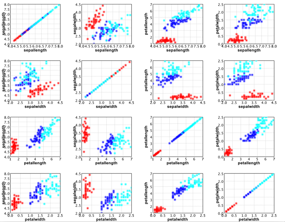
Line Chart
A line chart connects points by straight lines.
def line(data: Array[Array[Double]], style: Line.Style = Line.Style.SOLID, color: Color = Color.BLACK, mark: Char = ' ', label: String = null): Canvas public class LinePlot { public static LinePlot of(double[][] data, Line.Style style, Color color); public static LinePlot of(double[] y, Line.Style style, Color color); } Let's draw a heart with it!
val heart = -314 to 314 map { i => val t = i / 100.0 val x = 16 * pow(sin(t), 3) val y = 13 * cos(t) - 5 * cos(2*t) - 2 * cos(3*t) - cos(4*t) Array(x, y) } show(line(heart.toArray, color = RED)) import static java.lang.Math.*; double[][] heart = new double[200][2]; for (int i = 0; i < 200; i++) { double t = PI * (i - 100) / 100; heart[i][0] = 16 * pow(sin(t), 3); heart[i][1] = 13 * cos(t) - 5 * cos(2*t) - 2 * cos(3*t) - cos(4*t); } var figure = LinePlot.of(heart, Color.RED).figure(); var pane = new FigurePane(figure); pane.window(); 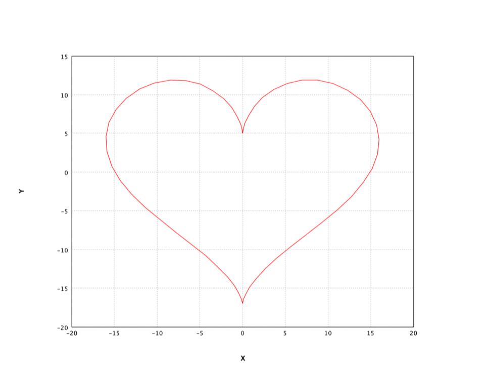
Box Plot
The box plot is a standardized way of displaying the distribution of data based on the five number summary: minimum, first quartile, median, third quartile, and maximum.
Box plots can be useful to display differences between populations without making any assumptions of the underlying statistical distribution: they are non-parametric. The spacings between the different parts of the box help indicate the degree of dispersion (spread) and skewness in the data, and identify outliers.
def boxplot(data: Array[Double]*): Canvas def boxplot(data: Array[Array[Double]], labels: Array[String]): Canvas public class BoxPlot { public BoxPlot(double[][] data, String[] labels); public static BoxPlot of(double[]... data); } Note that the parameter data is a matrix of which each row to create a box plot.
val groups = (iris("sepallength").toDoubleArray zip iris("class").toStringArray).groupBy(_._2) val labels = groups.keys.toArray val data = groups.values.map { a => a.map(_._1) }.toArray val canvas = boxplot(data, labels) canvas.figure.setAxisLabels("", "sepallength") show(canvas) String[] labels = ((smile.data.measure.NominalScale) iris.schema().field("class").measure()).levels(); double[][] data = new double[labels.length][]; for (int i = 0; i < data.length; i++) { var label = labels[i]; data[i] = iris.stream(). filter(row -> row.getString("class").equals(label)). mapToDouble(row -> row.getFloat("sepallength")). toArray(); } var figure = new BoxPlot(data, labels).figure(); figure.setAxisLabels("", "sepallength"); var pane = new FigurePane(figure); pane.window(); 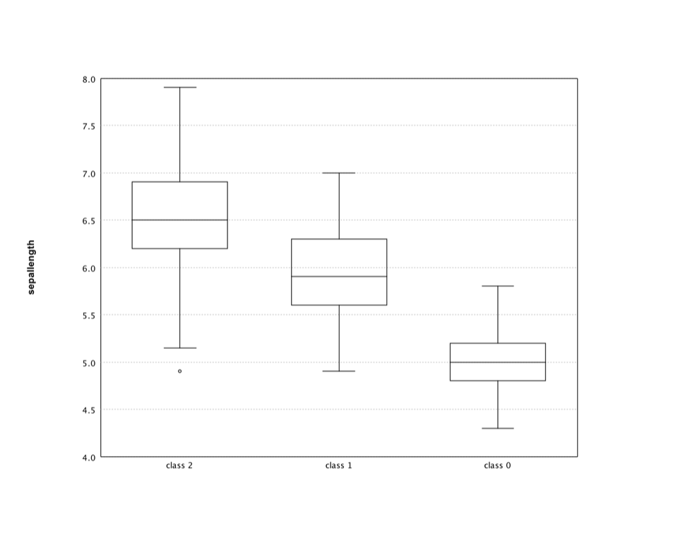
Histogram
A histogram is a graphical representation of the distribution of numerical data. The range of values is divided into a series of consecutive, non-overlapping intervals/bins. The bins must be adjacent, and are usually equal size.
def hist(data: Array[Double], k: Int = 10, prob: Boolean = false, color: Color = Color.BLUE): Canvas def hist(data: Array[Double], breaks: Array[Double], prob: Boolean, color: Color): Canvas public class Histogram { public static BarPlot of(double[] data); public static BarPlot of(double[] data, int k, boolean prob); public static BarPlot of(double[] data, int k, boolean prob, Color color); public static BarPlot of(double[] data, double[] breaks, boolean prob); public static BarPlot of(double[] data, double[] breaks, boolean prob, Color color); } where k is the number of bins (10 by default), or you can also specify an array of the breakpoints between bins.
Let's apply the histogram to an interesting data: the wisdom of crowds. The original experiment took place about a hundred years ago at a county fair in England. The fair had a guess the weight of the ox contest. Francis Galton calculated the average of all guesses, which is right to within one pound.
Recently, NPR Planet Money ran the experiment again. NPR posted a couple of pictures of a cow (named Penelope) and asked people to guess her weight. They got over 17,000 responses. The average of guesses was 1,287 pounds, which is pretty close to Penelope's weight 1,355 pounds.
val cow = read.csv("data/stat/cow.txt", header=false)("V1").toDoubleArray val canvas = hist(cow, 50) canvas.figure.setAxisLabels("Weight", "Probability") show(canvas) var cow = Read.csv("data/stat/cow.txt").column("V1").toDoubleArray(); var figure = Histogram.of(cow, 50, true).figure(); figure.setAxisLabels("Weight", "Probability"); var pane = new FigurePane(figure); pane.window(); 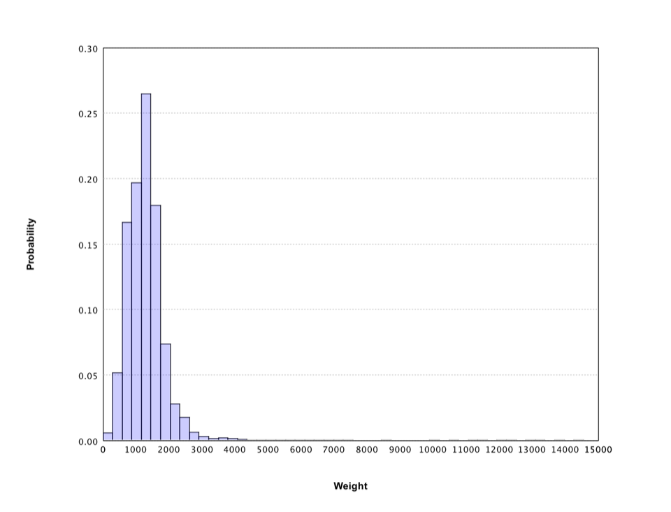
The histogram gives a rough sense of the distribution of crowd guess, which has a long tail. Filter out the weights over 3500 pounds, the histogram shows more details.
val canvas = hist(cow.filter(_ <= 3500), 50) canvas.figure.setAxisLabels("Weight", "Probability") show(canvas) var figure = Histogram.of(Arrays.stream(cow).filter(w -> w <= 3500).toArray(), 50, true).figure(); figure.setAxisLabels("Weight", "Probability"); var pane = new FigurePane(figure); pane.window(); 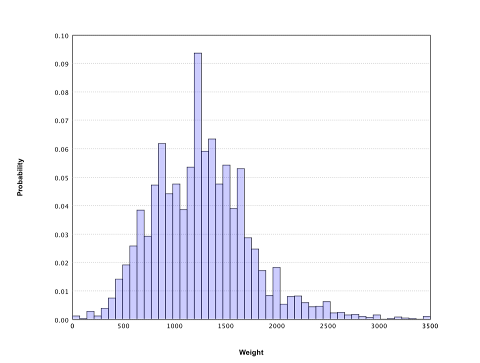
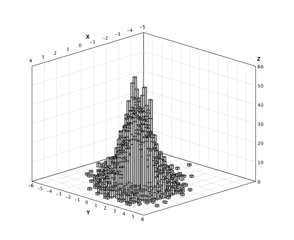
Smile also supports histograms that display the distribution of 2-dimensional data.
def hist3(data: Array[Array[Double]], xbins: Int = 10, ybins: Int = 10, prob: Boolean = false, palette: Array[Color] = Palette.jet(16)): Canvas public class Histogram3D { public static Histogram3D of(double[][] data); public static Histogram3D of(double[][] data, int nbins, Color[] palette); public static Histogram3D of(double[][] data, int nbins, boolean prob); public static Histogram3D of(double[][] data, int nbins, boolean prob, Color[] palette); } Here we generate a data set from a 2-dimensional Gaussian distribution.
val gauss = new MultivariateGaussianDistribution(Array(0.0, 0.0), Matrix.of(Array(Array(1.0, 0.6), Array(0.6, 2.0)))) val data = (0 until 10000) map { i: Int => gauss.rand } show(hist3(data.toArray, 50, 50)) double[] mu = {0.0, 0.0}; double[][] v = { {1.0, 0.6}, {0.6, 2.0} }; var gauss = new MultivariateGaussianDistribution(mu, Matrix.of(v)); var data = Stream.generate(gauss::rand).limit(10000).toArray(double[][]::new); var figure = Histogram3D.of(data, 50, false).figure(); var pane = new FigurePane(figure); pane.window(); The corresponding histogram looks like
Q-Q Plot
A Q–Q plot ("Q" stands for quantile) is a probability plot for comparing two probability distributions by plotting their quantiles against each other. A point (x, y) on the plot corresponds to one of the quantiles of the second distribution (y-coordinate) plotted against the same quantile of the first distribution (x-coordinate).
def qqplot(x: Array[Double]): Canvas def qqplot(x: Array[Double], d: Distribution): Canvas def qqplot(x: Array[Double], y: Array[Double]): Canvas def qqplot(x: Array[Int], d: DiscreteDistribution): Canvas def qqplot(x: Array[Int], y: Array[Int]): Canvas public class QQPlot { public static QQPlot of(double[] x); public static QQPlot of(double[] x, Distribution d); public static QQPlot of(double[] x, double[] y); public static QQPlot of(int[] x, DiscreteDistribution d); public static QQPlot of(int[] x, int[] y); } Smile supports the Q-Q plot of samples to a given distribution and also of two sample sets. The second distribution/samples is optional. If missing, we assume it the standard Gaussian distribution.
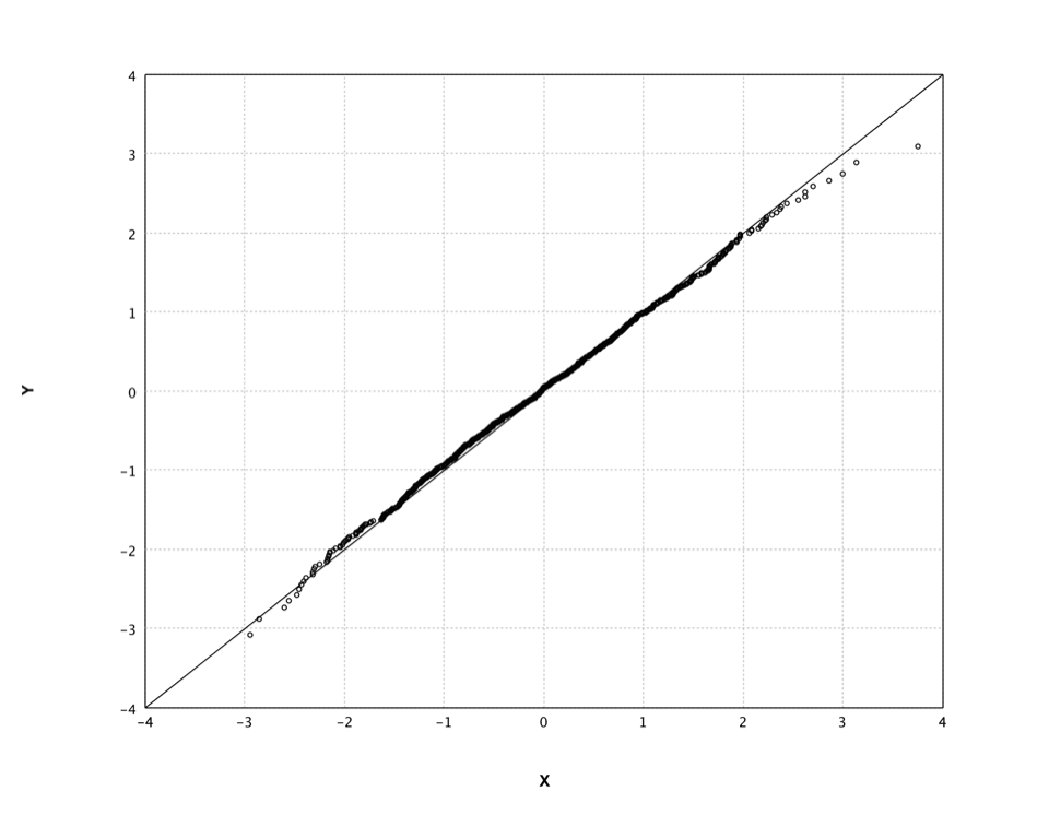
In what follows, we generate a random sample set from standard Gaussian distribution and draw its Q-Q plot.
val gauss = new GaussianDistribution(0.0, 1.0) val data = (0 until 1000) map { i: Int => gauss.rand } show(qqplot(data.toArray)) var gauss = new GaussianDistribution(0.0, 1.0); var data = DoubleStream.generate(gauss::rand).limit(1000).toArray(); var figure = QQPlot.of(data).figure(); var pane = new FigurePane(figure); pane.window(); In fact, this is also a good visual way to verify the quality of our random number generator.
Heatmap
A heat map is a graphical representation of data where the values in a matrix are represented as colors. In cluster analysis, researchers often employs the heat map by permuting the rows and the columns of a matrix to place similar values near each other according to the clustering.
def heatmap(z: Array[Array[Double]], palette: Array[Color] = Palette.jet(16)): Canvas def heatmap(x: Array[Double], y: Array[Double], z: Array[Array[Double]], palette: Array[Color]): Canvas def heatmap(rowLabels: Array[String], columnLabels: Array[String], z: Array[Array[Double]], palette: Array[Color]): Canvas public class Heatmap { public static Heatmap of(double[][] z); public static Heatmap of(double[][] z, int k); public static Heatmap of(double[] x, double[] y, double[][] z); public static Heatmap of(double[] x, double[] y, double[][] z, int k); public static Heatmap of(String[] rowLabels, String[] columnLabels, double[][] z); public static Heatmap of(String[] rowLabels, String[] columnLabels, double[][] z, int k); } where z is the matrix to display and the optional parameters x and y are the coordinates of data matrix cells, which must be in ascending order. Alternatively, one can also provide labels as the coordinates, which is a common practice in cluster analysis.
In what follows, we display the heat map of a matrix. We start with a small 4 x 4 matrix and enlarge it with bicubic interpolation. We also use the helper class Palette to generate the color scheme. This class provides many other color schemes.
// the matrix to display val z = Array( Array(1.0, 2.0, 4.0, 1.0), Array(6.0, 3.0, 5.0, 2.0), Array(4.0, 2.0, 1.0, 5.0), Array(5.0, 4.0, 2.0, 3.0) ) // make the matrix larger with bicubic interpolation val x = Array(0.0, 1.0, 2.0, 3.0) val y = Array(0.0, 1.0, 2.0, 3.0) val bicubic = new BicubicInterpolation(x, y, z) val Z = Array.ofDim[Double](101, 101) for (i <- 0 to 100) { for (j <- 0 to 100) Z(i)(j) = bicubic.interpolate(i * 0.03, j * 0.03) } show(heatmap(Z, Palette.jet(256))) // the matrix to display double[][] z = { {1.0, 2.0, 4.0, 1.0}, {6.0, 3.0, 5.0, 2.0}, {4.0, 2.0, 1.0, 5.0}, {5.0, 4.0, 2.0, 3.0} }; // make the matrix larger with bicubic interpolation double[] x = {0.0, 1.0, 2.0, 3.0}; double[] y = {0.0, 1.0, 2.0, 3.0}; var bicubic = new BicubicInterpolation(x, y, z); var Z = new double[101][101]; for (int i = 0; i <= 100; i++) { for (int j = 0; j <= 100; j++) Z[i][j] = bicubic.interpolate(i * 0.03, j * 0.03); } var figure = Heatmap.of(Z, Palette.jet(256)).figure(); var pane = new FigurePane(figure); pane.window(); 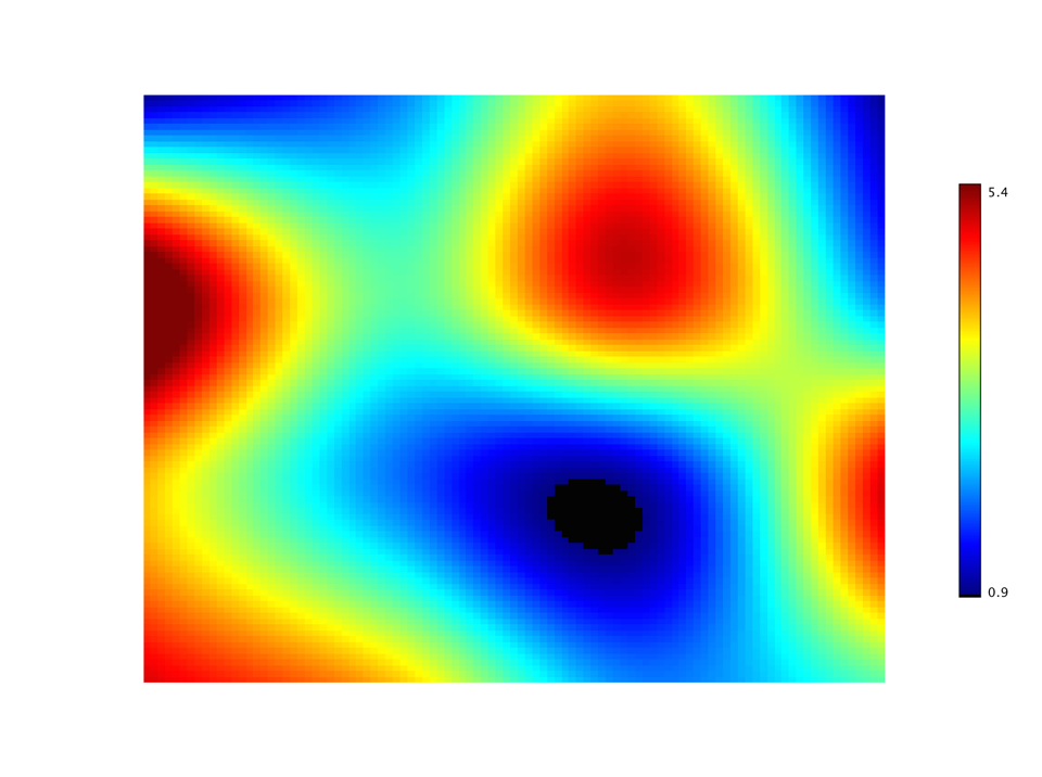
A special case of heat map is to draw the sparsity pattern of a matrix.
def spy(matrix: SparseMatrix, k: Int = 1): Canvas public class SparseMatrixPlot { public static SparseMatrixPlot of(SparseMatrix sparse); public static SparseMatrixPlot of(SparseMatrix sparse, int k); } The structure of sparse matrix is critical in solving linear systems.
val sparse = SparseMatrix.text(java.nio.file.Paths.get("data/matrix/mesh2em5.txt")) val canvas = spy(sparse) canvas.figure.setTitle("mesh2em5") show(canvas) var sparse = SparseMatrix.text(java.nio.file.Paths.get("data/matrix/mesh2em5.txt")); var figure = SparseMatrixPlot.of(sparse).figure(); figure.setTitle("mesh2em5"); var pane = new FigurePane(figure); pane.window(); 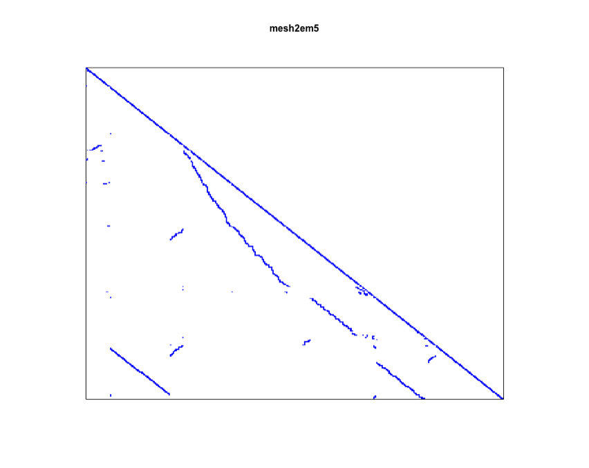
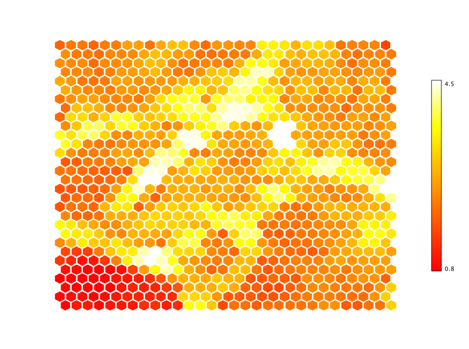
Another variant is the hex map where hexagon cells replace rectangle cells.
def hexmap(z: Array[Array[Double]], palette: Array[Color] = Palette.jet(16)): Canvas public class Hexmap { public static Hexmap of(double[][] z); public static Hexmap of(double[][] z, int k); public static Hexmap of(double[][] z, Color[] palette); } In machine learning, the hex map is often used to visualize self-organized map (SOM). An SOM is a type of artificial neural network that is trained using unsupervised learning to produce a low-dimensional (typically two-dimensional), discretized representation of the input space of the training samples. An SOM consists of components called nodes or neurons. Associated with each node are a weight vector of the same dimension as the input data vectors, and a position in the map space. The U-Matrix value of a particular node is the average distance between the node's weight vector and that of its closest neighbors. In practice, researchers often use the hex map to visualize the U-Matrix.
In the following example, we train and visualize a SOM on the USPS training data set with 30 x 30 nodes.
import smile.util.function._ val zip = read.csv("data/usps/zip.train", delimiter = " ", header = false) val x = zip.drop(0).toArray() val lattice = SOM.lattice(30, 30, x) val som = new SOM(lattice, TimeFunction.constant(0.1), Neighborhood.Gaussian(1, x.length * 10 / 4)) for (i <- 0 until 10) { MathEx.permutate(x.length).foreach { j => som.update(x(j)) } } show(hexmap(som.umatrix, Palette.heat(256))) var zip = Read.csv("data/usps/zip.train", CSVFormat.DEFAULT.withDelimiter(' ')); var x = zip.drop(0).toArray(); var lattice = SOM.lattice(30, 30, x); var som = new SOM(lattice, TimeFunction.constant(0.1), Neighborhood.Gaussian(1, x.length * 10 / 4)); for (int i = 0; i < 10; i++) { for (int j : MathEx.permutate(x.length)) { som.update(x[j]); } } var figure = Hexmap.of(som.umatrix(), Palette.heat(256)).figure(); var pane = new FigurePane(figure); pane.window(); In the hex map, areas of low neighbour distance indicate groups of nodes that are similar. Areas with large distances indicate the nodes are much more dissimilar, and indicate natural boundaries between node clusters.
Contour
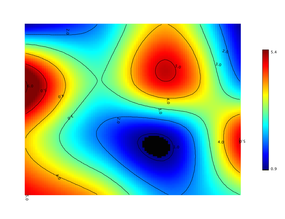
A contour plot represents a 3-dimensional surface by plotting constant z slices, called contours, on a 2-dimensional format. That is, given a value for z, lines are drawn for connecting the (x, y) coordinates where that z value occurs.
def contour(z: Array[Array[Double]]): Canvas def contour(z: Array[Array[Double]], levels: Array[Double]): Canvas def contour(x: Array[Double], y: Array[Double], z: Array[Array[Double]]): Canvas def contour(x: Array[Double], y: Array[Double], z: Array[Array[Double]], levels: Array[Double]): Canvas public class Contour { public static Contour of(double[][] z); public static Contour of(double[][] z, int numLevels); public static Contour of(double[] x, double[] y, double[][] z); public static Contour of(double[] x, double[] y, double[][] z, int numLevels); } Similar to heatmap, the parameters x and y are the coordinates of data matrix cells, which must be in ascending order. The slice values can be automatically determined from the data, or provided through the parameter levels.
Contours are often jointly used with the heat map. In the following example, we add the contour lines to the previous heat map exampl.
val canvas = heatmap(Z, Palette.jet(256)) canvas.figure.add(Contour.of(Z)) show(canvas) var figure = Heatmap.of(Z, 256).figure(); figure.add(Contour.of(Z)); var pane = new FigurePane(figure); pane.window(); This example also shows how to mix multiple plots together. Besides using the plot functions directly, one can also construct plots with Java classes and add them to existing a plot canvas.
Surface
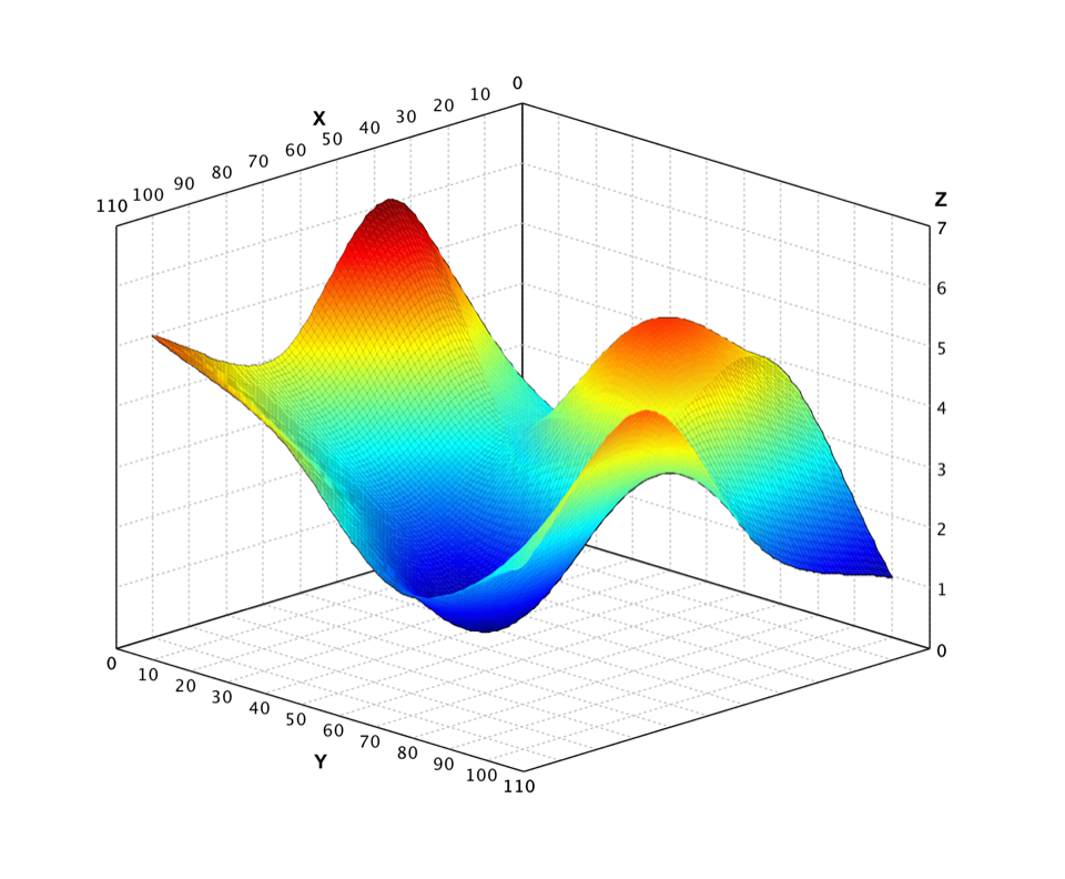
Besides heat map and contour, we can also visualize a matrix with the three-dimensional shaded surface.
def surface(z: Array[Array[Double]], palette: Array[Color] = Palette.jet(16)): Canvas def surface(x: Array[Double], y: Array[Double], z: Array[Array[Double]], palette: Array[Color]): Canvas public class Surface { public static Surface of(double[][] z); public static Surface of(double[][] z, Color[] palette); public static Surface of(double[] x, double[] y, double[][] z); public static Surface of(double[] x, double[] y, double[][] z, Color[] palette); } The usage is similar with heatmap and contour functions.
show(surface(Z, Palette.jet(256, 1.0f))) var figure = Surface.of(Z, Palette.jet(256, 1.0f)).figure(); var pane = new FigurePane(figure); pane.window(); The surface of same example data is shown as
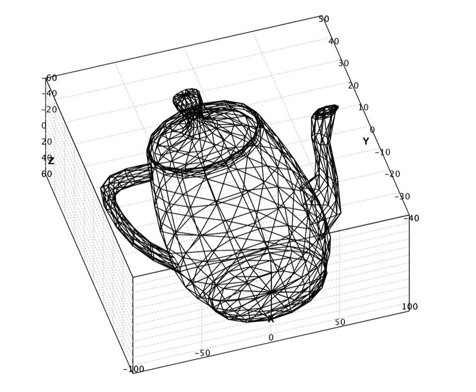
Wireframe
The wireframe model is a visual presentation of a three-dimensional physical object. A wireframe model consists of two tables, the vertex table and the edge table. Each entry of the vertex table records a vertex and its coordinate values, while each entry of the edge table has two components giving the two incident vertices of that edge.
def wireframe(vertices: Array[Array[Double]], edges: Array[Array[Int]]): Canvas public class Wireframe { public static Wireframe of(double[][] vertices, int[][] edges); } where vertices is an n x 2 or n x 3 array which are coordinates of n vertices, and edges is an m x 2 array of which each row is the vertex indices of two end points of each edge.
val (vertices, edges) = read.wavefront("data/wavefront/teapot.obj") show(wireframe(vertices, edges)) The above code draws the wireframe of a teapot.