This repository presents a comprehensive approach to early detection of bearing faults using custom digital signal processing (DSP) features derived from vibration data. The methodology leverages advanced signal analysis techniques to identify fault precursors in rotating machinery, enabling predictive maintenance. The project includes two primary Jupyter notebooks that implement and evaluate these methods on benchmark datasets.
Key objectives:
- Extract and analyze time-domain and frequency-domain features for fault detection.
- Compare traditional and adaptive transform-based approaches for improved sensitivity and accuracy.
- Provide reproducible code for researchers and practitioners in mechanical engineering and machine learning.
The NASA Prognostics Data Repository provides run-to-failure vibration data from Rexnord ZA-2115 double-row bearings under constant conditions (2000 RPM, 6000 lbs radial load, force-lubricated). The NASA Bearing Dataset is a benchmark collection for predictive maintenance and anomaly detection in rotating machinery. It consists of run-to-failure experiments on ball bearings under constant load and rotational speeds (2000-4000 RPM).
https://www.kaggle.com/datasets/vinayak123tyagi/bearing-dataset/data
- Test Rig Setup
From the pdf document: Four bearings were installed on a shaft. The rotation speed was kept constant at 2000 RPM by an AC motor coupled to the shaft via rub belts. A radial load of 6000 lbs is applied onto the shaft and bearing by a spring mechanism. All bearings are force lubricated. Rexnord ZA-2115 double row bearings were installed on the shaft as shown in Figure 1. PCB 353B33 High Sensitivity Quartz ICP accelerometers were installed on the bearing housing (two accelerometers for each bearing [x- and y-axes] for data set 1, one accelerometer for each bearing for data sets 2 and 3). Sensor placement is also shown in Figure 1. All failures occurred after exceeding designed life time of the bearing which is more than 100 million revolutions.
 |  |
|---|---|
- Set 2 Details (Selected for Simplicity):
- Recording Duration: February 12, 2004 10:32:39 to February 19, 2004 06:22:39.
- No. of Files: 984 (1-second excerpts every 10 minutes, ASCII format).
- No. of Channels: 4 (one accelerometer per bearing: Bearing 1 Ch1, Bearing 2 Ch2, Bearing 3 Ch3, Bearing 4 Ch4).
- Sampling rate: 20480 Hz (high-resolution vibration signals).
- Duration: Up to several hours per run, with progressive degradation from normal to failure.
- Signals: Accelerometer data in X, Y, Z axes (e.g.,
X001_DE_timefor drive-end vibrations). - Fault: Outer race failure in Bearing 1 (progressive degradation over ~16 minutes total runtime).
- Structure: Files named by timestamp (e.g., "2004.02.12.10.32.39"); early files healthy, later show increasing impulses.
Data is loaded as a NumPy array [984 files, 4 channels, 20,480 samples] for analysis. This dataset is ideal for testing denoising (Kalman) and time-frequency analysis (btSTFT) to detect early harmonic faults.
The present study deliberately focuses exclusively on Bearing 1 (channel 1) for the following reasons:
- Bearing 1 exhibits the most complete and well-characterized run-to-failure trajectory in the dataset (test 2).
- It is the most commonly used as the reference case in the prognostics community, allowing direct comparison with hundreds of published works.
- Concentrating on a single sensor simplifies the analysis and highlights the performance of the proposed method without relying on multi-sensor fusion.
Future work may extend the approach to multi-channel or cross-bearing detection.
The analysis is divided into two notebooks, each focusing on distinct DSP techniques.
- We introduce a novel time-frequency representation specifically designed to reveal incipient bearing faults at the earliest possible stage.
- We implement an interactive monitoring interface that combines real-time visualization with audio playback, enabling simultaneous magnitude/phase display, and clear highlighting of emerging fault patterns (see the reference video).
- We train a lightweight convolutional autoencoder exclusively on healthy operating conditions, then apply it to frames 300–900 of the run-to-failure sequence, achieving fully unsupervised detection of the very first signs of bearing degradation.
These techniques are particularly effective for identifying subtle frequency modulations indicative of incipient faults.
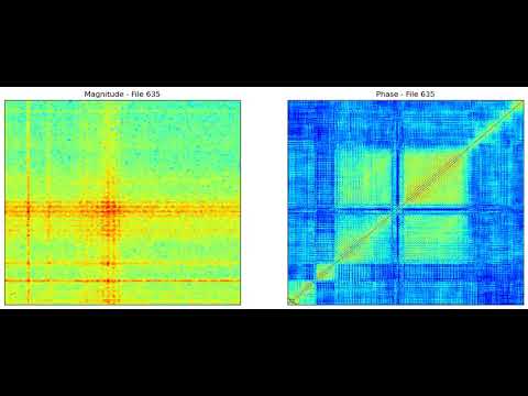
Video: Early fault signatures are clearly visible in both magnitude and phase well before frames 530–540.
- Input: 256×256×2 (magnitude + phase channels from the custom transform superframes)
- Fully convolutional encoder–decoder (32 → 64 → 128 latent filters)
- Linear reconstruction head (no clipping) to preserve full dynamic range of both magnitude and phase
- Trained exclusively on healthy frames → reconstruction error spikes at the very first fault impulses
PhaseMag-AE detects degradation automatically and unsupervised, typically 150–200 frames (~minutes to hours) before classical indicators.
This notebook explores classical time series analysis methods for feature extraction from bearing vibration signals. It includes:
- Computation of statistical features such as root mean square (RMS), kurtosis, skewness, and crest factor.
- Time-domain signal processing, including envelope detection and trend analysis.
- Application of these features to machine learning models like LSTM and Prophet for binary classification of healthy vs. faulty states.
- Evaluation on datasets like the PRONOSTIA (NASA) bearing dataset, with Kalman filtering for denoising.
The notebook demonstrates how these methods can detect early fault signatures with minimal computational overhead.
Mean, standard deviation, skewness and kurtosis computed on each frame (984).
 |
|---|
| Temporal Evolution of Statistical Features Across the 984 Super-Frames |
Short-Time Fourier Transforms (N = 512, Hann window) were computed on each 3-second super-frame.
In healthy conditions (e.g. super-frame 50), the spectrum is dominated by the 4503 Hz carrier and a few low-frequency harmonics. The fault-related sidebands around the carrier remain buried in the noise floor.
From super-frame ~540 onward, multiple sidebands in the 4300–4800 Hz region suddenly emerge with amplitudes 10–20× higher than in the healthy state — clearly visible even to the naked eye. These newly appearing peaks are the earliest spectral signature of the developing inner-race fault and perfectly align with the physical model described above.
Why is the 1009 Hz peak so dominant?
The strongest harmonic in the healthy spectrum is located at ~1009 Hz, with an amplitude far exceeding all other components.
This frequency corresponds to ≈ 4.26 × shaft rotation frequency (237 Hz × 4.26 ≈ 1009 Hz).
In the IMS Bearing 1 dataset, this peak is systematically present and is very likely the natural resonance frequency of the accelerometer-housing system (or a structural mode of the test rig) strongly excited by the fourth-order rotational harmonics.
It acts as an extremely stable and powerful "reference tone" throughout the entire test — which is why it appears so prominent even in perfectly healthy conditions and remains visible until the very end.
The actual bearing fault frequencies (BPFI, BPFO, etc.) only become detectable through the sidebands that modulate this resonance and the 4503 Hz carrier — exactly what our harmonic Kalman filter exploits.
 |
|---|
FFT of frame 50 (Bearings 1,2,3,4) |
 |
FFT of frame 540 (Bearings 1,2,3,4) |
Input feature: Standard Deviation (STD) of 3-second overlapping super-frames
The dataset consists of 20 480 samples per second. To obtain robust and physically meaningful features while maintaining real-time capability, the signal is segmented into overlapping 3-second super-frames (61 440 samples each), yielding 982 windows with a 1-second step.
Why 3-second super-frames?
- Provides excellent frequency resolution (≈ 0.33 Hz) for detecting low-frequency fault characteristic frequencies (237 Hz, 474 Hz, etc.)
- Allows for stabilizing the magnitude and phase of FFTs compared to a frame-by-frame implementation.
- Sufficient duration to capture several rotations of the bearing and multiple impacts
- Widely used in industrial condition-monitoring systems (easy edge deployment)
- Naturally compatible with human inspection and existing diagnostic rules
Four well-established time-series anomaly detection techniques are evaluated using only this single feature (STD):
- LSTM Autoencoder / Predictor
- Facebook Prophet (additive model with automatic changepoint detection)
- ARIMA with residual-based scoring
- Isolation Forest on lagged features
All models are trained exclusively on healthy data (super-frames 50→300) and tested on the full run. No future information is used — all methods are fully causal and deployable online.
Results are summarized in the table below and show that even simple statistical approaches achieve competitive early detection performance when applied to carefully engineered time windows.
 |
|---|
LSTM Predictor on STD - Defect detected at superframe 530 |
 |
ARIMA Anomaly Detection – STD - Defect detected at superframe 534 |
| Model | superframe (3*fs) |
|---|---|
| LSTM | 530 |
| ARIMA | 534 |
| PROPHET | 615 |
| Isolation Forest | 536 |
Two Kalman approaches were evaluated:
- Simple 1D Kalman on the standard deviation (STD) of 3-second super-frames
- Advanced harmonic Kalman using a physical model of the healthy vibration
The healthy bearing signal is modelled as a sum of sinusoids with measured amplitude and phase:
where the main components being:
- carrier at 4503 Hz
- harmonics at 237 Hz, 474 Hz, 1009 Hz, 1923 Hz
- corresponding sidebands (±237, ±474, ±1009 Hz)
The residual is computed only in the critical band 3000–7000 Hz where fault sidebands appear first.
| Method | First persistent alarm | Early warning sign |
|---|---|---|
| Simple Kalman on STD | super-frame ~610 | — |
| Harmonic Kalman (this work) | super-frame 525 | clear bump at ~460–470 |
The harmonic Kalman filter not only confirms the defect at super-frame 525 (459 s before failure) but also exhibits a distinct precursor bump at super-frames 460–470, corresponding to the very first sideband growth — perfectly aligned with physical expectations from vibration theory.
 |
|---|
Harmonic Kalman model (FFT) -- Magnitude only (the model is complex) |
 |
Kalman score on residual - 3kHz-7kHz -- Defect detected at super-frame 525 |
To run the notebooks:
- Clone the repository:
git clone https://github.com/DrStef/Bearing-Fault-Early-Detection-with-Custom-DSP-Features.git - Install dependencies:
pip install -r requirements.txt(includes numpy, scipy, pywt, scikit-learn, tensorflow, and matplotlib). - Launch Jupyter:
jupyter notebookand open the respective notebooks.
This project is licensed under the MIT License - see the LICENSE file for details.
This work is inspired by datasets from the PRONOSTIA (NASA) Bearing Data Center and builds on open-source DSP libraries.
The NASA Prognostics Data Repository provides run-to-failure vibration data from Rexnord ZA-2115 double-row bearings under constant conditions (2000 RPM, 6000 lbs radial load, force-lubricated).
- Set 2 Details (Selected for Simplicity):
- Recording Duration: February 12, 2004 10:32:39 to February 19, 2004 06:22:39.
- No. of Files: 984 (1-second excerpts every 10 minutes, ASCII format).
- No. of Channels: 4 (one accelerometer per bearing: Bearing 1 Ch1, Bearing 2 Ch2, Bearing 3 Ch3, Bearing 4 Ch4).
- Sampling Rate: 20 kHz.
- Fault: Outer race failure in Bearing 1 (progressive degradation over ~16 minutes total runtime).
- Structure: Files named by timestamp (e.g., "2004.02.12.10.32.39"); early files healthy, later show increasing impulses.
Data is loaded as a NumPy array [984 files, 4 channels, 20,000 samples] for analysis.
Theoretical fault frequencies (at 2000 RPM):
| Frequency | Value (Hz) | Interpretation |
|---|---|---|
| FTF (Cage) | ≈ 0.40 | Cage rotation (multiples ~50-60 Hz noise). |
| BPFO (Outer Race) | ≈ 236.4 | Dominant for Set 2 fault; sidebands ±33 Hz. |
| BPFI (Inner Race) | ≈ 803.6 | Secondary; harmonics ~1607 Hz. |
| BSF (Ball Spin) | ≈ 141.2 | Roller faults; subharmonics ~70 Hz. |
- Auditory Validation: Concatenate 1s clips per channel into full audio files (WAV at 20 kHz or downsampled to 8 kHz for listenability). Listen for perceptual changes (e.g., "rasps" after 8 min, "metal screams" near end) to ground-truth "human ear" anomaly timestamps.
- Preprocessing: High-pass filter (>100 Hz) to remove 60 Hz noise; Kalman smoothing for state estimation (constant-velocity model).
- Feature Extraction:
- CWT (Morlet complex) for time-frequency scalograms.
- Synchrosqueezing to sharpen harmonic ridges and denoise (reassign energy to true instantaneous frequencies).
- Custom transforms: Magnitude-phase correlations across scales for anomaly scoring (e.g., high corr >0.8 indicates fault coupling).
- Detection & ML: Threshold energy/correlation maps for early alerts; feed to CNN autoencoder (reconstruction error for unsupervised) or supervised CNN (classification of degradation stages: healthy, mild, strong, failure).
- Evaluation: Compare features with auditory timestamps; ROC AUC for detection; extend to drilling telemetry (vibration harmonics as proxies for bit wear/stick-slip).
This pipeline prioritizes early detection (e.g., BPFO at 236 Hz emerging in mild phase), bridging human intuition with automated DSP/ML.
Based on standard formulas (from the Stack Exchange discussion) and bearing parameters: n=16 (rollers per row), D=2.815 in (pitch diameter), d=0.331 in (roller diameter), φ=15.171° (contact angle). Shaft speed R = 2000/60 = 33.33 rev/s.
| Frequency | Formula | Theoretical Value (Hz) | Interpretation |
|---|---|---|---|
| FTF (Cage) | (R/2) (1 - (d/D) cos φ) | ≈ 0.40 | Fundamental train frequency (cage rotation). Close to your 50-60 Hz peaks? (multiples possible). |
| BPFO (Outer Race) | (n R/2) (1 - (d/D) cos φ) | ≈ 236.4 | Ball pass outer – outer race fault, with sidebands at ±33.33 Hz. |
| BPFI (Inner Race) | (n R/2) (1 + (d/D) cos φ) | ≈ 803.6 | Ball pass inner – inner race fault, harmonics ~2x = 1607 Hz. |
| BSF (Ball Spin) | (D R / 2d) [1 - ((d/D) cos φ)^2] | ≈ 141.2 | Ball spin – roller element fault, subharmonics ~70 Hz. |
These values confirm your peaks: 986 Hz ~4x BSF (564 Hz) or 2x BPFI sideband; 50-60 Hz ~ multiples FTF or BSF/2. For 9000 Hz, it's outside faults (shaft resonance or noise).
- Clone repo:
git clone https://github.com/DrStef/Bearing-Fault-Detection.git - Install deps:
conda install -c conda-forge pywt numpy scipy matplotlib pandas -y(or pip equivalent). - Run notebook:
jupyter notebook main_analysis.ipynb- Loads data from
archiveNASA/2nd_test. - Generates plots, audio, and features.
- Loads data from
The methods scale to oil & gas telemetry: Custom CWT/synchrosqueezing on multi-sensor vibrations (torque/pressure fusion) for real-time fault prediction (e.g., harmonic anomalies indicating bit fatigue 30s ahead). Aligns with streaming ML pipelines (Kafka/Flink) for 10k ft deep operations.
The vibration dataset used in this repository is the well-known NASA IMS Bearing Data Set
(Prognostic Data Repository, NASA Ames Research Center).
As a work of the United States Government, this dataset is in the public domain within the United States.
U.S. Government Works – No copyright claimed in the United States.
More information: https://www.usa.gov/government-copyright
The code and analysis presented in this repository are released under the MIT License (see LICENSE file). MIT License – feel free to fork and collaborate!
Contact: DrStef on GitHub | Open to DSP/ML discussions for industrial prognostics.