Jupyter Examples
- Standard plot
- Interactive Plot using D3js
- Interactive Plot using Bokeh
- LaTex
- Inline images
- IFrame
- More examples
- Paste the following code in a python file
- Execute it (either selecting the code or using the
Run cellcode lens). - The result is a static graph displayed in the
Resultswindow
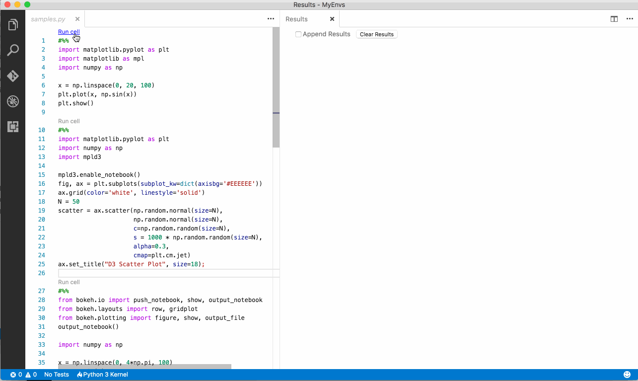
#%% import matplotlib.pyplot as plt import matplotlib as mpl import numpy as np x = np.linspace(0, 20, 100) plt.plot(x, np.sin(x)) plt.show() - Paste the following code in a python file
- Execute it (either selecting the code or using the
Run cellcode lens). - The result is an interactive displayed in the
Resultswindow - Check here for more infor on D3js
Note: Hover the mouse over the graph and a toolbar should appear allowing you to interact with the graph
#%% import matplotlib.pyplot as plt import numpy as np import mpld3 mpld3.enable_notebook() fig, ax = plt.subplots(subplot_kw=dict(axisbg='#EEEEEE')) ax.grid(color='white', linestyle='solid') N = 50 scatter = ax.scatter(np.random.normal(size=N), np.random.normal(size=N), c=np.random.random(size=N), s = 1000 * np.random.random(size=N), alpha=0.3, cmap=plt.cm.jet) ax.set_title("D3 Scatter Plot", size=18);- Paste the following code in a python file
- Execute it (either selecting the code or using the
Run cellcode lens). - The result is an interactive displayed in the
Resultswindow - Check here for more info on Bokeh graphs
Note: Use the toolbar next to the graph image, to interact with the graph.
#%% from bokeh.io import push_notebook, show, output_notebook from bokeh.layouts import row, gridplot from bokeh.plotting import figure, show, output_file output_notebook() import numpy as np x = np.linspace(0, 4*np.pi, 100) y = np.sin(x) TOOLS = "pan,wheel_zoom,box_zoom,reset,save,box_select" p1 = figure(title="Legend Example", tools=TOOLS) p1.circle(x, y, legend="sin(x)") p1.circle(x, 2*y, legend="2*sin(x)", color="orange") p1.circle(x, 3*y, legend="3*sin(x)", color="green") show(p1)- Check here for more info on LaTex
#%% from IPython.display import Latex Latex('''The mass-energy equivalence is described by the famous equation $$E=mc^2$$ discovered in 1905 by Albert Einstein. In natural units ($c$ = 1), the formula expresses the identity \\begin{equation} E=m \\end{equation}''') #%% from IPython.display import Image Image('http://jakevdp.github.com/figures/xkcd_version.png')#%% from IPython.core.display import HTML HTML("<iframe src='http://www.ncdc.noaa.gov/oa/satellite/satelliteseye/cyclones/pfctstorm91/pfctstorm.html' width='750' height='600'></iframe>")- Interactive Matplotlib graphs using d3js (mpld3)
- Interactive Bokeh graphs
- LaTex