GETPIVOTDATA

This function returns visible data from a Pivot Table. It queries the pivot table and gets the specific data based on the pivot table structure, instead of cell references. The main advantage of using this function is that it ensures that the correct data is returned, even if the pivot table layout is changed.

Syntax

=GETPIVOTDATA(data_field, pivot_table, [field1, item1, field2, item2], ...)

Arguments

This function has the following arguments:

Arguments	Descriptions
data_field	The name of the PivotTable field that contains the data you want to retrieve. This needs to be in double-quotes.
pivot_table	A reference to any cell, range of cells, or named range of cells in a PivotTable. This information is used to determine which PivotTable contains the data that you want to retrieve.
field1, item1, field2, item2..	[Optional] Up to 126 pairs of field names and item names that describe the data that you want to retrieve. The pairs can be in any order.

Usage

You can enter the GETPIVOTDATA function by using = (the equal sign) in the cell in which you want to return the value. You can also use this function with other functions.

Remarks

The following points hold true while working with the GETPIVOTTABLE function:

#REF! error value occurs in the following cases:
- If the given pivot_table reference is not related to the pivot table.
- If an invalid field for the data_field, [field], or [item] arguments is provided.
- If the arguments do not describe a visible field, or if they include a report filter in which the filtered data is not displayed.
When there is a sigma value, the data_field will contain calc type, otherwise, it will use the field name only.

Return value

Returns visible data from a pivot table.

Examples

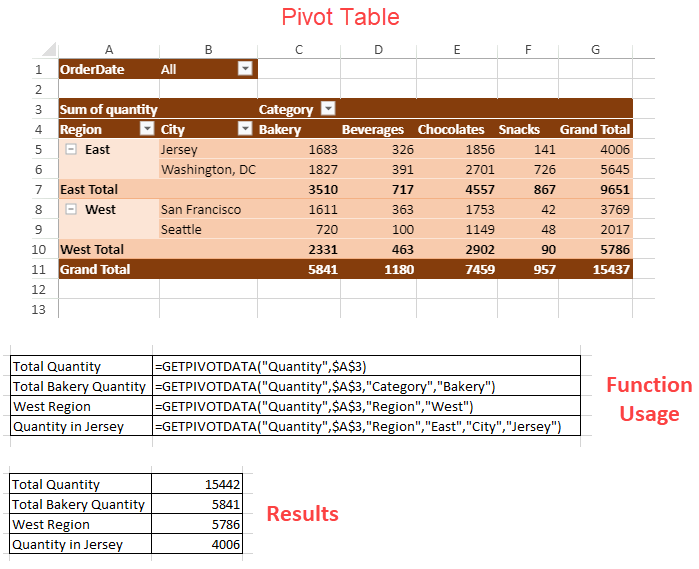
The following images show the usage of the GETPIVOTDATA function.

The following code sample shows the usage of the GETPIVOTDATA function.

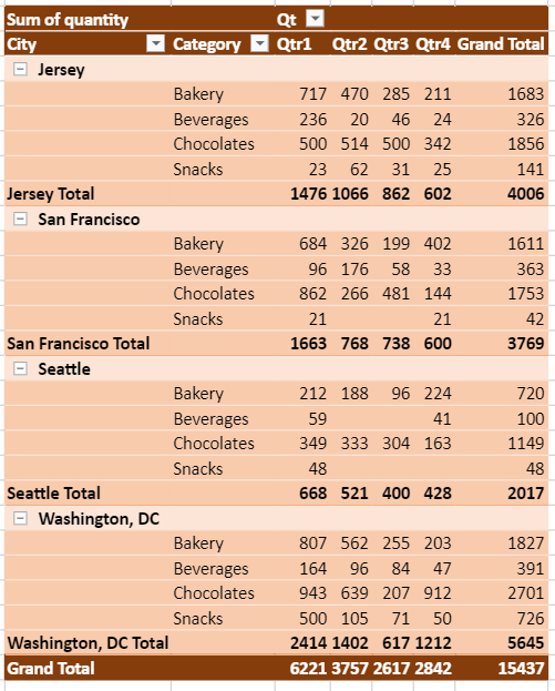
$(document).ready(function () { // initializing Spread var spread = new GC.Spread.Sheets.Workbook(document.getElementById('ss'), { sheetCount: 2 }); spread.suspendPaint(); // get sheets var pivotLayoutSheet = spread.getSheet(0); var dataSourceSheet = spread.getSheet(1); // set sheet name pivotLayoutSheet.name("PivotLayout"); dataSourceSheet.name("DataSource"); // set row count dataSourceSheet.setRowCount(245); // set datasource dataSourceSheet.setArray(0, 0, pivotDB_UseCase); // add table to dataSourceSheet dataSourceSheet.tables.add('tableSales', 0, 0, 245, 8); spread.resumePaint(); // initialize pivottable initPivotTable(pivotLayoutSheet); // auto fit columns in both the sheets autoFit(pivotLayoutSheet); autoFit(dataSourceSheet); }); function initPivotTable(sheet) { // add pivottable var myPivotTable = sheet.pivotTables.add("myPivotTable", "tableSales", 0, 0, GC.Spread.Pivot.PivotTableLayoutType.tabular, GC.Spread.Pivot.PivotTableThemes.dark3); myPivotTable.suspendLayout(); // show rowHeader and columnHeader for PivotTable myPivotTable.options.showRowHeader = true; myPivotTable.options.showColumnHeader = true; // add column fields myPivotTable.add("Category", "Category", GC.Spread.Pivot.PivotTableFieldType.columnField); // add row fields myPivotTable.add("Region", "Region", GC.Spread.Pivot.PivotTableFieldType.rowField); myPivotTable.add("City", "City", GC.Spread.Pivot.PivotTableFieldType.rowField); // add value field with SubtotalType Sum myPivotTable.add("Quantity", "Sum of quantity", GC.Spread.Pivot.PivotTableFieldType.valueField, GC.Pivot.SubtotalType.sum); // add filter field myPivotTable.add("OrderDate", "OrderDate", GC.Spread.Pivot.PivotTableFieldType.filterField); var formula1 = '=GETPIVOTDATA("Quantity",$A$3)'; sheet.setValue(3, 10, 'Total Quantity'); sheet.setStyle(3, 10, 'introSec'); sheet.setFormula(3, 11, formula1); var formula2 = '=GETPIVOTDATA("Quantity",$A$3,"Category","Bakery")'; sheet.setValue(4, 10, 'Total Bakery Quantity'); sheet.setStyle(4, 10, 'introSec'); sheet.setFormula(4, 11, formula2); var formula3 = '=GETPIVOTDATA("Quantity",$A$3,"Region","West")'; sheet.setValue(5, 10, 'West Region'); sheet.setStyle(5, 10, 'introSec'); sheet.setFormula(5, 11, formula3); var formula4 = '=GETPIVOTDATA("Quantity",$A$3,"Region","East","City","Jersey")'; sheet.setValue(6, 10, 'Quantity in Jersey'); sheet.setStyle(6, 10, 'introSec'); sheet.setFormula(6, 11, formula4); myPivotTable.resumeLayout(); return myPivotTable; } function autoFit(sheet) { // auto fit columns let columnCount = sheet.getColumnCount(); for (let i = 0; i < columnCount; i++) { sheet.autoFitColumn(i); } }

The GETPIVOTDATA function also supports spilling, which means, it can populate multiple cells with its results. However, the allowDynamicArray property should be set to true to observe the spilling results. The below image shows a pivot table that will be used to extract some meaningful results using the GETPIVOTDATA function.

The below image shows the output when the GETPIVOTDATA function is used in the above pivot table and the result is spilled to multiple cells.

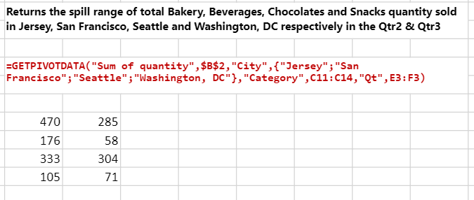
The following code sample shows the usage of the GETPIVOTDATA function to get results that spill to multiple cells.

function setGetPivotDataFunction(sheet) { spread.options.allowDynamicArray = true; var formula = '=GETPIVOTDATA("Sum of quantity",$B$2,"City",{"Jersey";"San Francisco";"Seattle";"Washington, DC"},"Category",C11:C14,"Qt",E3:F3)'; sheet.setStyle(1, 9, 'introSec'); sheet.addSpan(1, 9, 2, 8, GC.Spread.Sheets.SheetArea.viewport); sheet.setValue(1, 9, 'Returns the spill range of total Bakery, Beverages, Chocolates and Snacks quantity sold in Jersey, San Francisco, Seattle and Washington, DC respectively in the Qtr2 & Qtr3'); sheet.getCell(1, 9).wordWrap(true); sheet.setStyle(4, 9, 'formula'); sheet.addSpan(4, 9, 2, 8, GC.Spread.Sheets.SheetArea.viewport); sheet.getCell(4, 9).wordWrap(true); sheet.setValue(4, 9, formula); sheet.setFormula(7, 9, formula); }