Deep Neural Networks Backward module

L-Model Backward module:

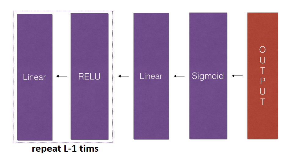
In this part, we will implement the backward function for the whole network. Recall that when we implemented the L_model_forward function, we stored a cache containing a cache at each iteration (X, W, b, and z). In the backpropagation module, we will use those variables to compute the gradients. Therefore, in the L_model_forward function, we will iterate through all the hidden layers backward, starting from layer L. In each step, we will use the cached values for layer l to backpropagate through layer l. The figure below shows the backward pass.

To backpropagate through this network, we know that the output is:

$A^{\left[L\right]}=\sigma \left(Z^{\left[L\right]}\right)$

Our code needs to compute:

$dAL=\frac{\partial L}{\partial A^{\left[L\right]}}$

To do so, we'll use this formula (derived using calculus which you don't need to remember):

# derivative of cost with respect to AL dAL = - (np.divide(Y, AL) - np.divide(1 - Y, 1 - AL))

We can then use this post-activation gradient dAL to keep going backward. As seen in the figure above, we can now feed in dAL into the LINEAR->SIGMOID backward function we implemented (which will use the cached values stored by the L_model_forward function). After that, we will have to use a for loop to iterate through all the other layers using the LINEAR->RELU backward function. We should store each dA, dW, and db in the grads dictionary. To do so, we'll use this formula:

$grads["dW"+str(l\left)\right]=d{W}^{\left[l\right]}$

For example, for l=3 this would store dW^[l] in grads["dW3"].

Code for our linear_backward function:

Arguments:

AL - probability vector, the output of the forward propagation L_model_forward();
Y - true "label" vector (containing 0 if non-cat, 1 if cat);
caches - list of caches containing:
1. every cache of linear_activation_forward() with "relu" (it's caches[l], for l in range(L-1) i.e l = 0...L-2);
2. the cache of linear_activation_forward() with "sigmoid" (it's caches[L-1]).

Return:

grads - A dictionary with the gradients:
grads["dA" + str(l)] = ...
grads["dW" + str(l)] = ...
grads["db" + str(l)] = ...

def L_model_backward(AL, Y, caches): grads = {} # the number of layers L = len(caches) m = AL.shape[1] # after this line, Y is the same shape as AL Y = Y.reshape(AL.shape) # Initializing the backpropagation dAL = - (np.divide(Y, AL) - np.divide(1 - Y, 1 - AL)) # Lth layer (SIGMOID -> LINEAR) gradients. Inputs: "dAL, current_cache". Outputs: "grads["dAL-1"], grads["dWL"], grads["dbL"] current_cache = caches[L-1] grads["dA" + str(L-1)], grads["dW" + str(L)], grads["db" + str(L)] = linear_activation_backward(dAL, current_cache, "sigmoid") # Loop from l=L-2 to l=0 for l in reversed(range(L-1)): # lth layer: (RELU -> LINEAR) gradients. # Inputs: "grads["dA" + str(l + 1)], current_cache". # Outputs: "grads["dA" + str(l)] , grads["dW" + str(l + 1)] , grads["db" + str(l + 1)] current_cache = caches[l] dA_prev_temp, dW_temp, db_temp = linear_activation_backward(grads["dA"+str(l+1)], current_cache, "relu") grads["dA" + str(l)] = dA_prev_temp grads["dW" + str(l + 1)] = dW_temp grads["db" + str(l + 1)] = db_temp return grads

Update Parameters module:

In this section, we will update the parameters of the model using gradient descent:

$$\begin{gathered} W^{\left[l\right]}=W^{\left[l\right]}-\alpha d{W}^{\left[l\right]} \\ {b}^{\left[l\right]}=b^{\left[l\right]}-\alpha d{b}^{\left[l\right]} \end{gathered}$$

here α is the learning rate. After computing the updated parameters, we'll store them in the parameters dictionary.

Code for our update_parameters function:

Arguments:

parameters - python dictionary containing our parameters.
Grads - python dictionary containing our gradients, output of L_model_backward.

Return:

parameters - python dictionary containing our updated parameters:
parameters["W" + str(l)] = ...
parameters["b" + str(l)] = ...

def update_parameters(parameters, grads, learning_rate):	# number of layers in the neural network L = len(parameters) // 2 # Update rule for each parameter for l in range(L): parameters["W" + str(l+1)] = parameters["W" + str(l+1)] - learning_rate*grads["dW" + str(l+1)] parameters["b" + str(l+1)] = parameters["b" + str(l+1)] - learning_rate*grads["db" + str(l+1)] return parameters

Conclusion: