Unit V -Graphical Models in artificial intelligence and machine learning

Graphical Models Prepared By: Nivetha Department of Computer Science and Engineering

Graphical Models • A graphical model is a probabilistic model for which a graph expresses the conditional dependence structure between random variables. • It provides a language to facilitate communication between a domain expert and a statistician, provide flexible and modular definitions of families of probability distributions, and are amenable to scalable computational techniques • Graphical models in machine learning are a powerful framework used to represent and reason about the dependencies between variables. • These models provide a structured way to visualize and compute joint probabilities for a set of variables in complex systems, which is useful for tasks like prediction, decision making, and inference.

Graphical Models • The Graphical model (GM) is a branch of ML which uses a graph to represent a domain problem • Probabilistic graphical modeling combines both probability and graph theory • Also called as Bayesian networks, belief networks or probabilistic networks • Consists of graph structure-Nodes and arcs • Two categories — Bayesian networks and Markov networks

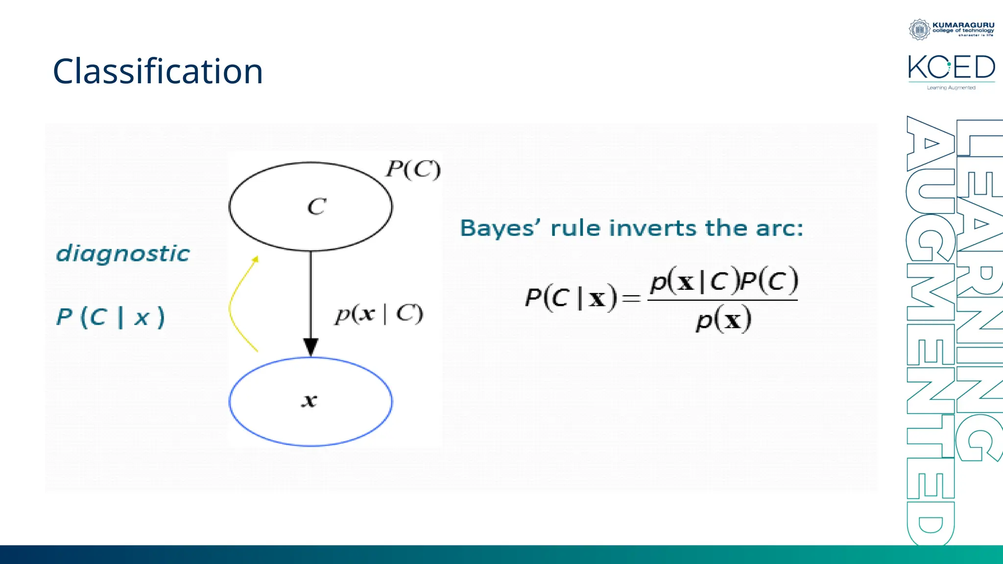
Graphical Models • Each node corresponds to a random variable, X, and has a value corresponding to the probability of the random variable, P(X). • If there is a directed arc from node X to node Y, this indicates that X has a direct influence on Y. • This influence is specified by the conditional probability directed acyclic P(Y|X). • Bayesian -The network is a directed acyclic graph (DAG); namely, these are graph no cycles. • The nodes and the arcs between the nodes define the structure of the network, and the conditional probabilities are the parameters given the structure.

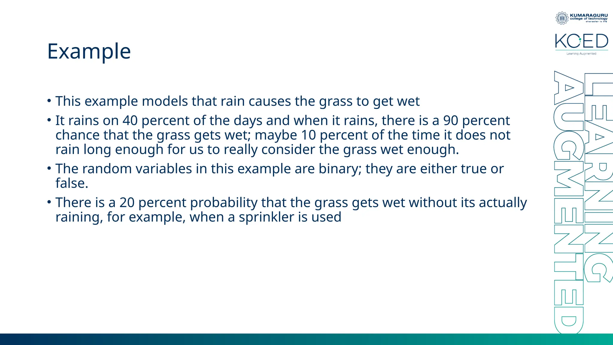
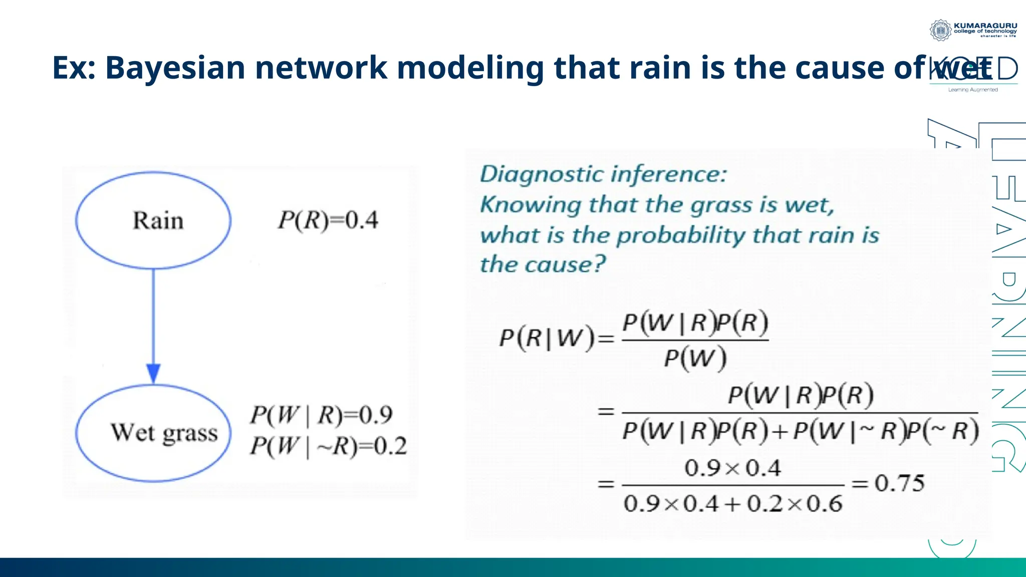
Example • This example models that rain causes the grass to get wet • It rains on 40 percent of the days and when it rains, there is a 90 percent chance that the grass gets wet; maybe 10 percent of the time it does not rain long enough for us to really consider the grass wet enough. • The random variables in this example are binary; they are either true or false. • There is a 20 percent probability that the grass gets wet without its actually raining, for example, when a sprinkler is used

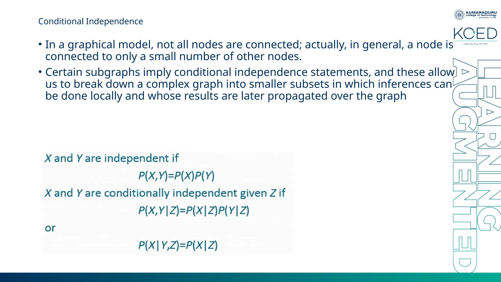
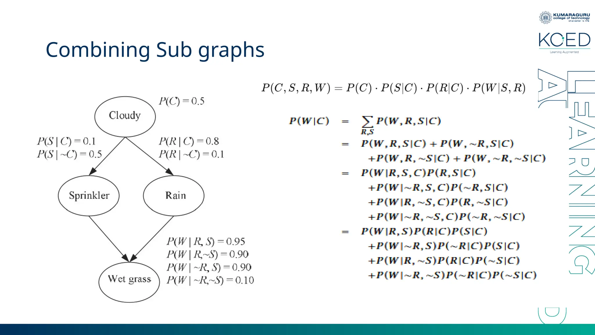
Ex: Bayesian network modeling that rain is the cause of wet

Conditional Independence • In a graphical model, not all nodes are connected; actually, in general, a node is connected to only a small number of other nodes. • Certain subgraphs imply conditional independence statements, and these allow us to break down a complex graph into smaller subsets in which inferences can be done locally and whose results are later propagated over the graph

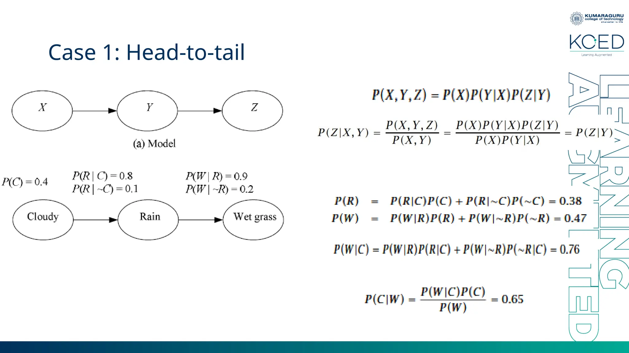
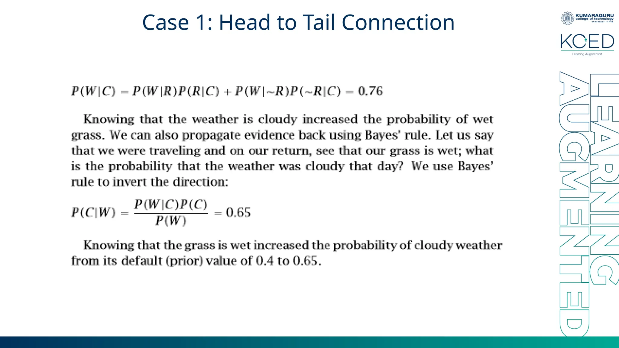
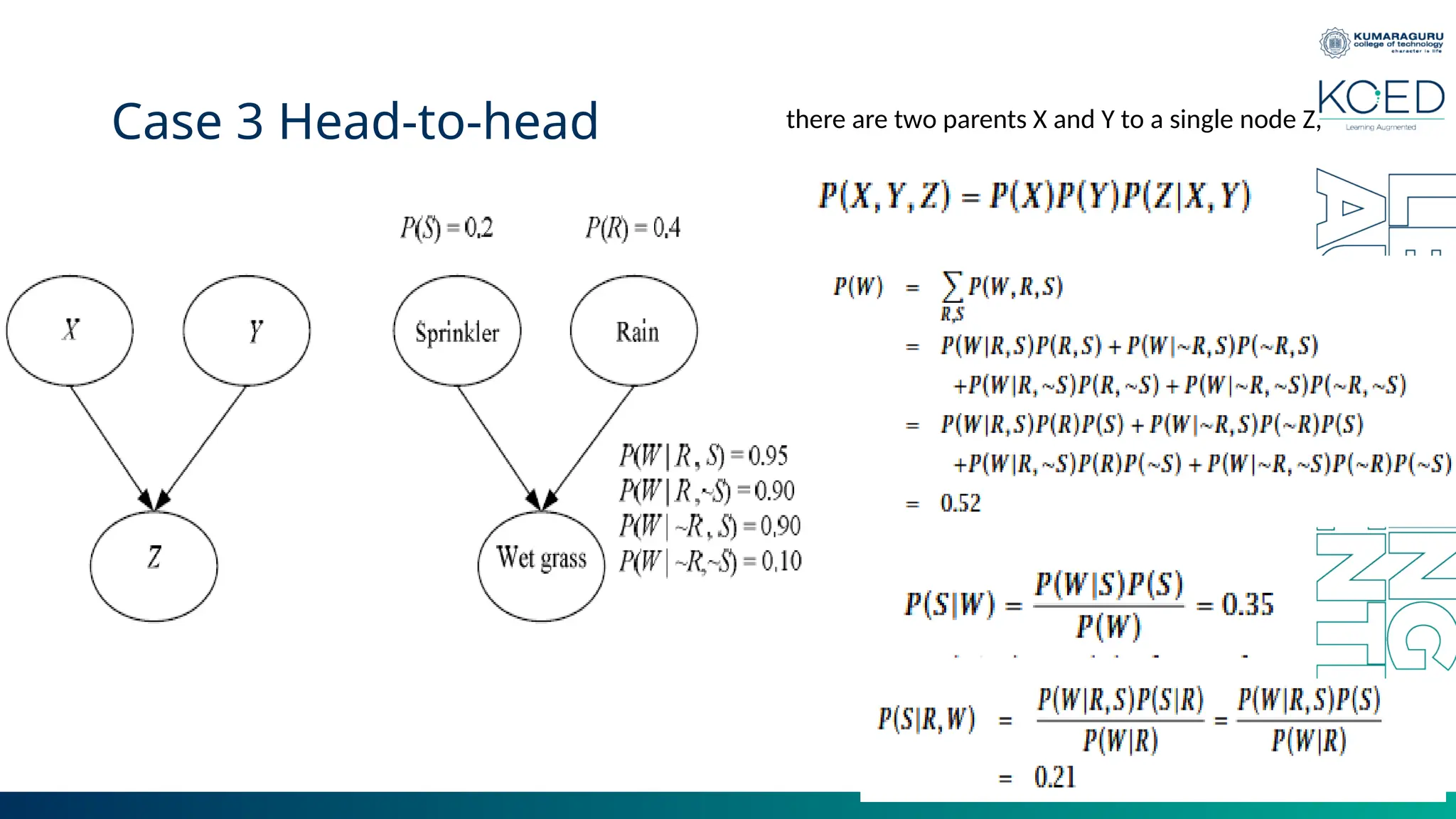
Canonical Cases for Conditional Independence • Head-to-tail Connection • Tail-to-Tail Connection • Head-to-Head Connection

Canonical Cases for Conditional Independence Case 1: Head-to-tail Connection •Three events may be connected serially, as seen in ﬁgure . We see here that X and Z are independent given Y: Knowing Y tells Z everything; knowing the state of X does not add any extra knowledge for Z; we write P(Z|Y,X)= P(Z|Y). We say that Y blocks the path from X to Z, or in other words, it separates them in the sense that if Y is removed, there is no path between X to Z. In this case, the joint is written as

Case 1: Head to Tail Connection

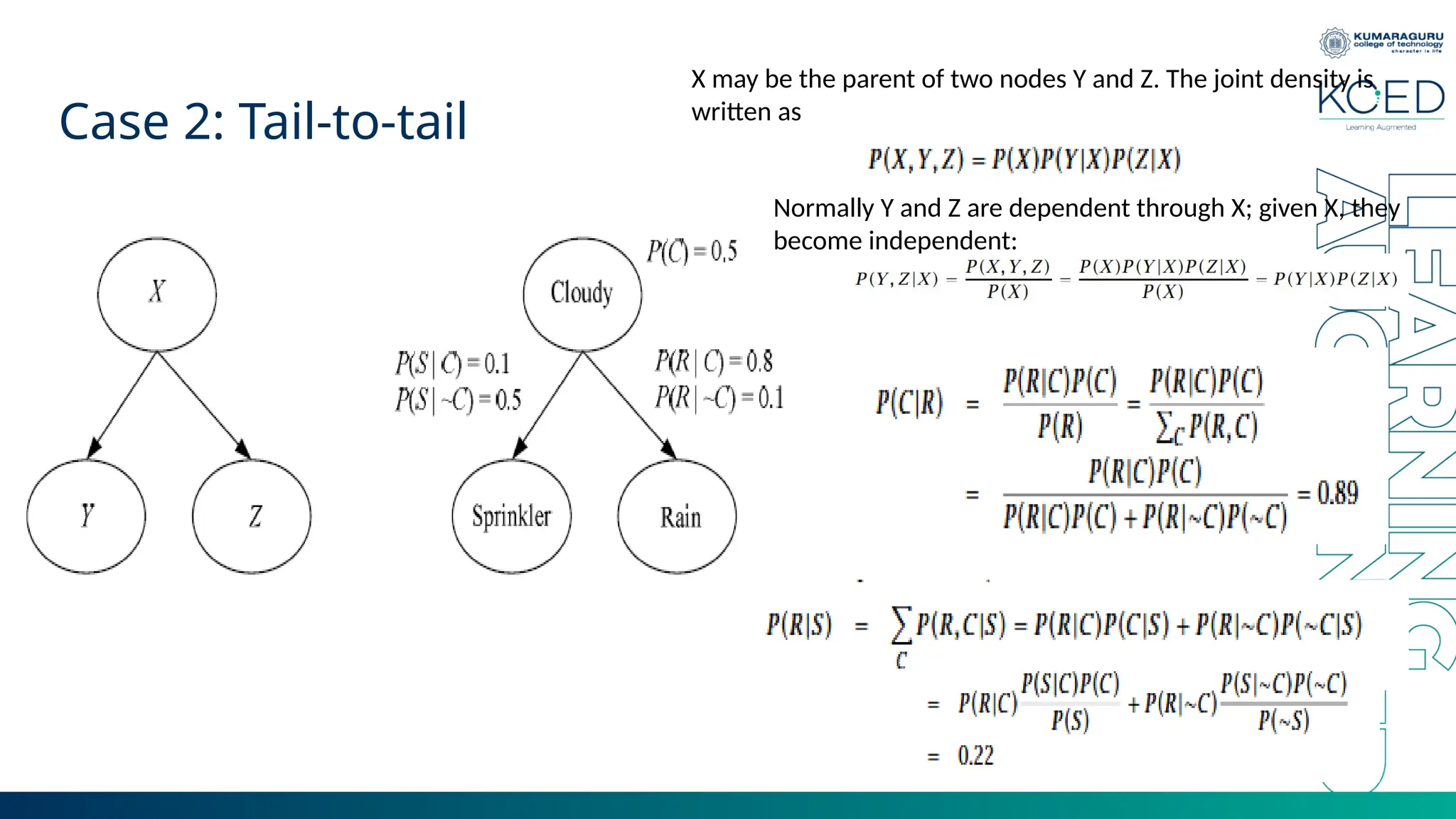
Case 2: Tail-to-tail X may be the parent of two nodes Y and Z. The joint density is written as Normally Y and Z are dependent through X; given X, they become independent:

Case 3 Head-to-head there are two parents X and Y to a single node Z,

Advantages • No of variables stored is less • we do not need to designate explicitly certain variables as input and certain others as output.

Example Graphical Model • Naïve Bayes Classifier • Hidden Markov model

Example Graphical Model Naive Bayes’ Classiﬁer Hidden Markov Model

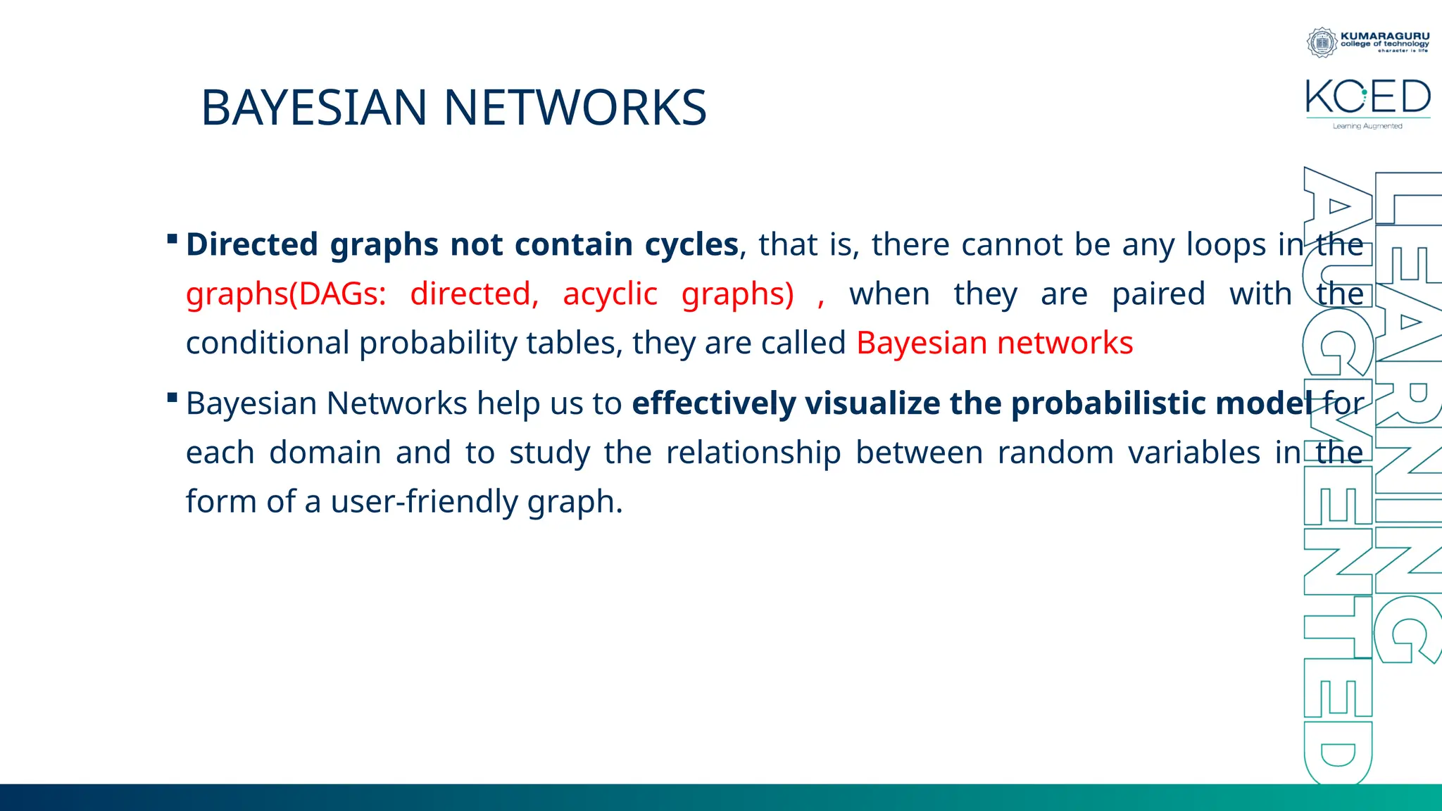
BAYESIAN NETWORKS  Directed graphs not contain cycles, that is, there cannot be any loops in the graphs(DAGs: directed, acyclic graphs) , when they are paired with the conditional probability tables, they are called Bayesian networks  Bayesian Networks help us to effectively visualize the probabilistic model for each domain and to study the relationship between random variables in the form of a user-friendly graph.

Why Bayes Network?  Bayes optimal classifier is too costly to apply  Naïve Bayes makes overly restrictive assumptions.  But all variables are rarely completely independent.  Bayes network represents conditional independence relations among the features.  Representation of causal relations makes the representation and inference efficient.

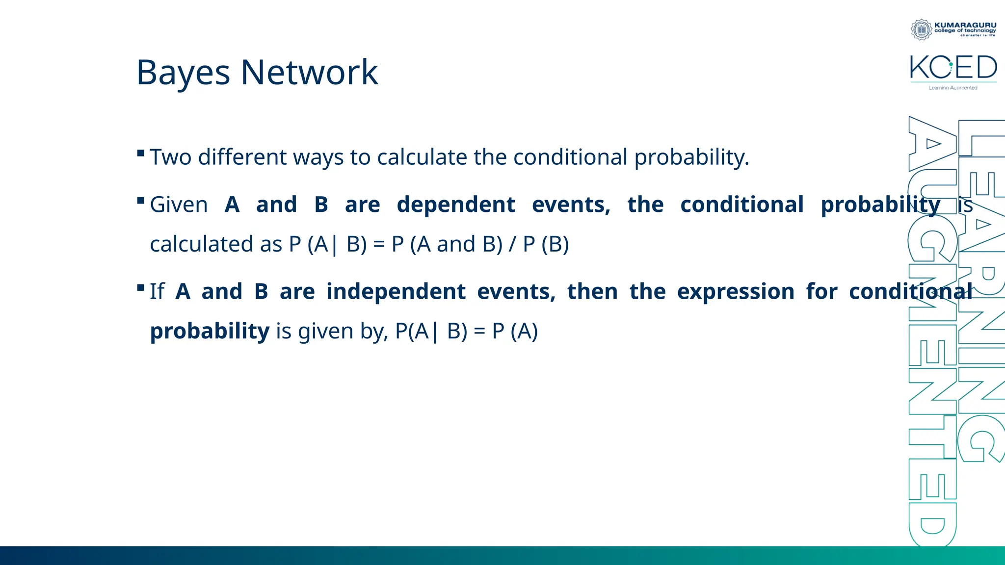
Bayes Network  Two different ways to calculate the conditional probability.  Given A and B are dependent events, the conditional probability is calculated as P (A| B) = P (A and B) / P (B)  If A and B are independent events, then the expression for conditional probability is given by, P(A| B) = P (A)

Bayesian Network – example 1 o The probability of a random variable depends on his parents. oBayesian network models capture both conditionally dependent and conditionally independent relationships between random variables.  Create a Bayesian Network that will model the marks of a student in his examination

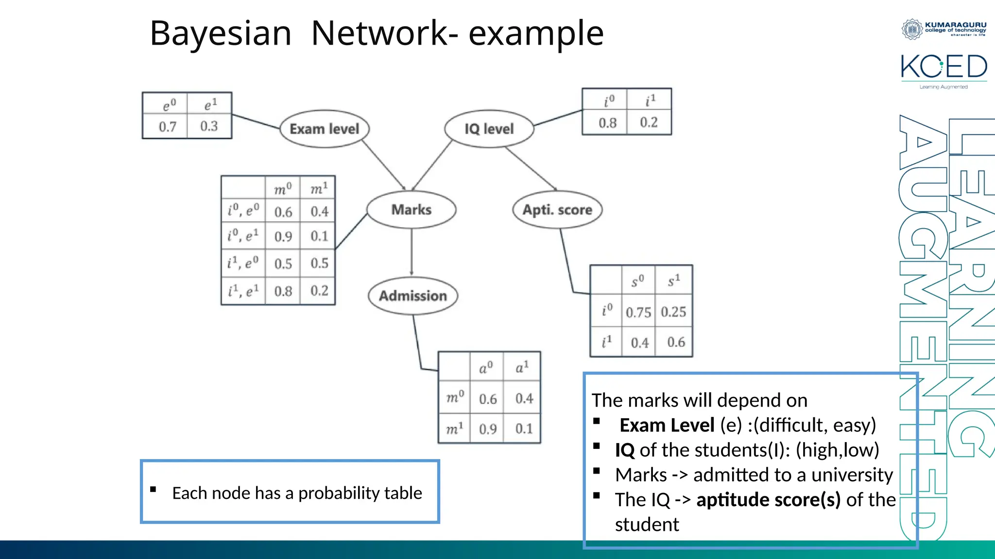
Bayesian Network- example The marks will depend on  Exam Level (e) :(difficult, easy)  IQ of the students(I): (high,low)  Marks -> admitted to a university  The IQ -> aptitude score(s) of the student  Each node has a probability table

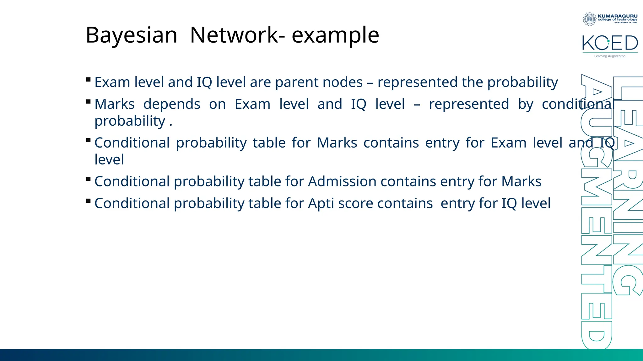
Bayesian Network- example  Exam level and IQ level are parent nodes – represented the probability  Marks depends on Exam level and IQ level – represented by conditional probability .  Conditional probability table for Marks contains entry for Exam level and IQ level  Conditional probability table for Admission contains entry for Marks  Conditional probability table for Apti score contains entry for IQ level

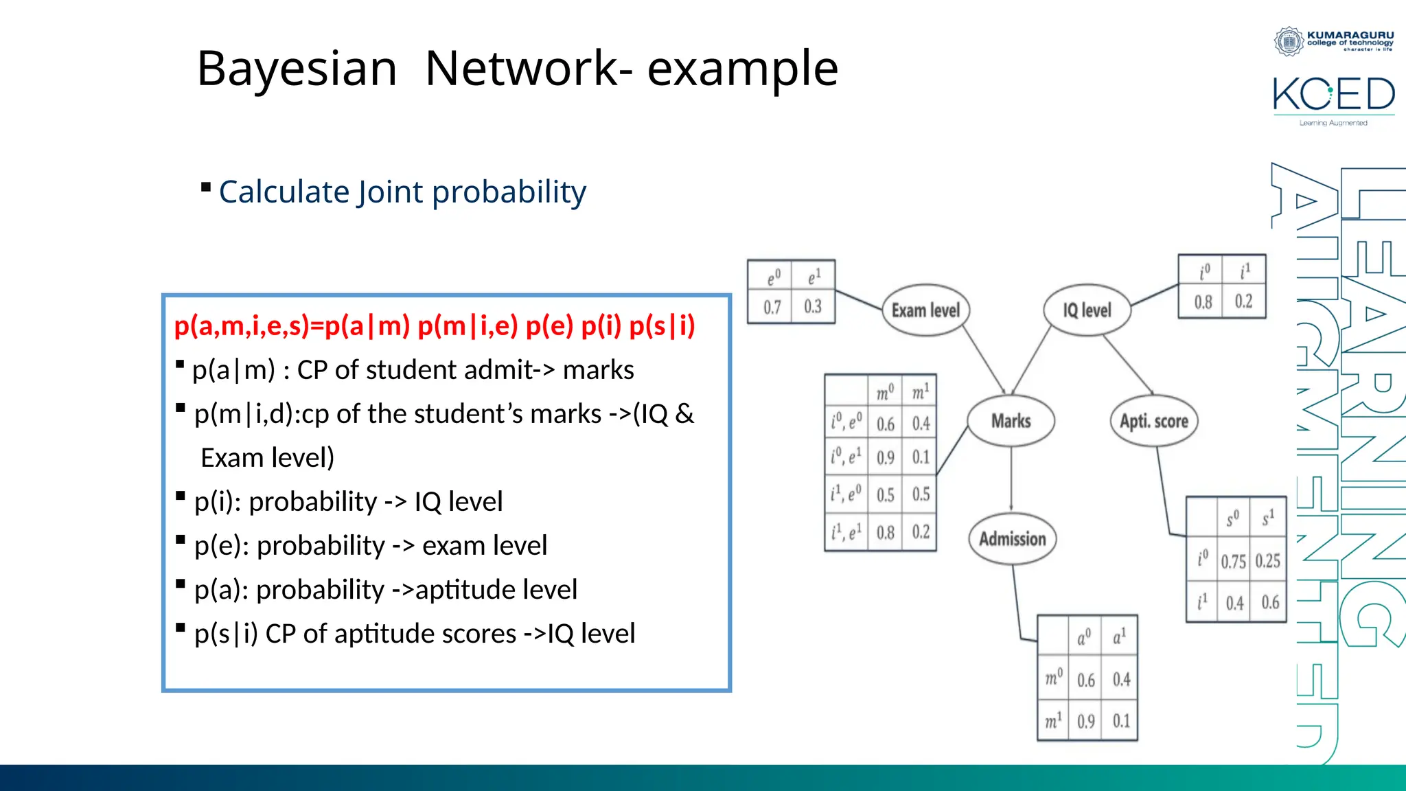
Bayesian Network- example  Calculate Joint probability p(a,m,i,e,s)=p(a|m) p(m|i,e) p(e) p(i) p(s|i)  p(a|m) : CP of student admit-> marks  p(m|i,d):cp of the student’s marks ->(IQ & Exam level)  p(i): probability -> IQ level  p(e): probability -> exam level  p(a): probability ->aptitude level  p(s|i) CP of aptitude scores ->IQ level

Bayesian Network- example Calculate the probability that in spite of the exam level being difficult, the student having a low IQ level and a low Aptitude Score, manages to pass the exam and secure admission to the university. Joint Probability Distribution can be written as P[a=1, m=1, i=0, e=1, s=0] From the above Conditional Probability tables, the values for the given conditions are fed to the formula and is calculated as below. P[a=1, m=1, i=0, e=0, s=0] = P(a=1 | m=1) . P(m=1 | i=0, e=1) . P(i=0) . P(e=1) . P(s=0 | i=0) = 0.1 * 0.1 * 0.8 * 0.3 * 0.75 = 0.0018

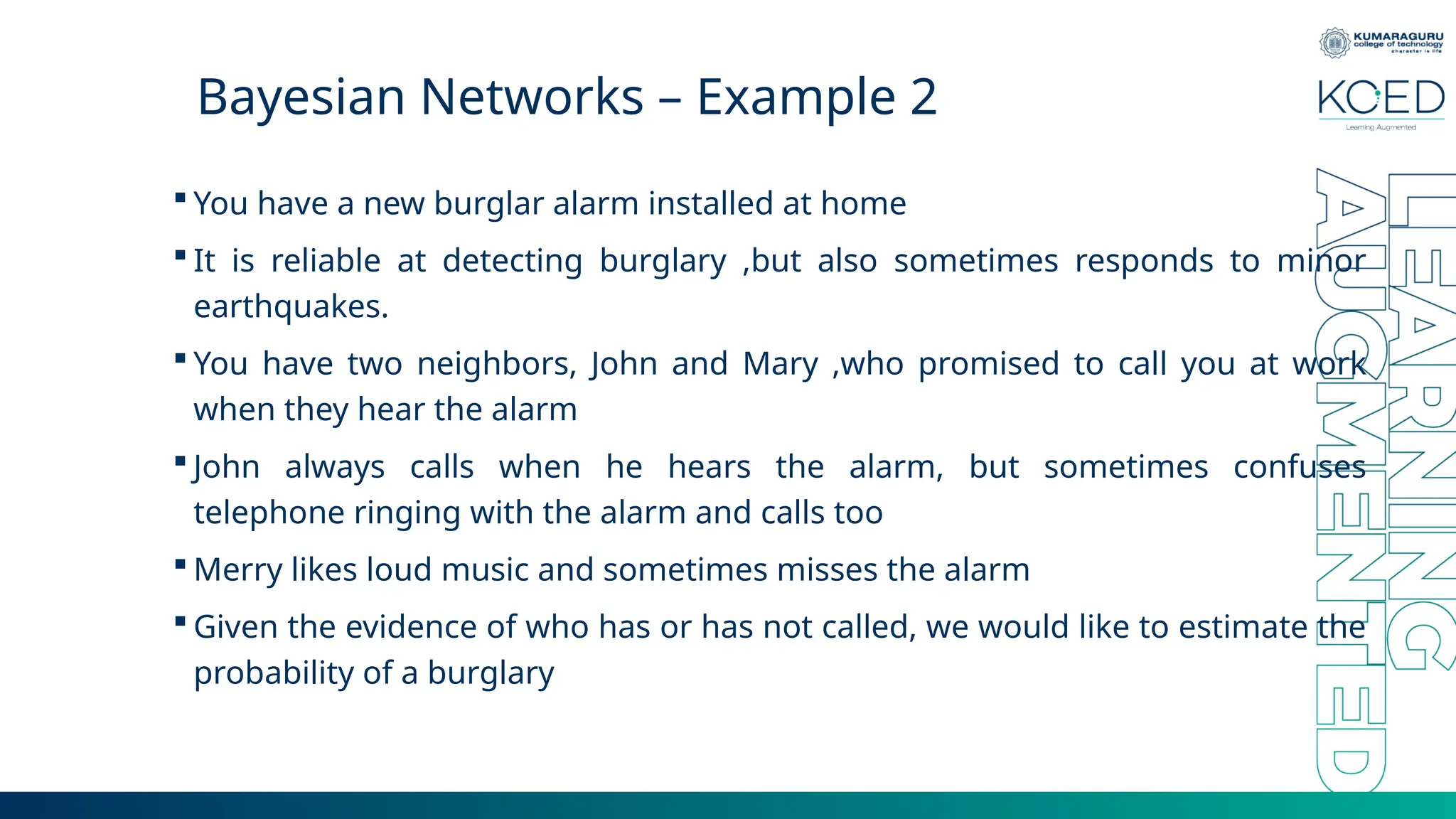
Bayesian Networks – Example 2  You have a new burglar alarm installed at home  It is reliable at detecting burglary ,but also sometimes responds to minor earthquakes.  You have two neighbors, John and Mary ,who promised to call you at work when they hear the alarm  John always calls when he hears the alarm, but sometimes confuses telephone ringing with the alarm and calls too  Merry likes loud music and sometimes misses the alarm  Given the evidence of who has or has not called, we would like to estimate the probability of a burglary

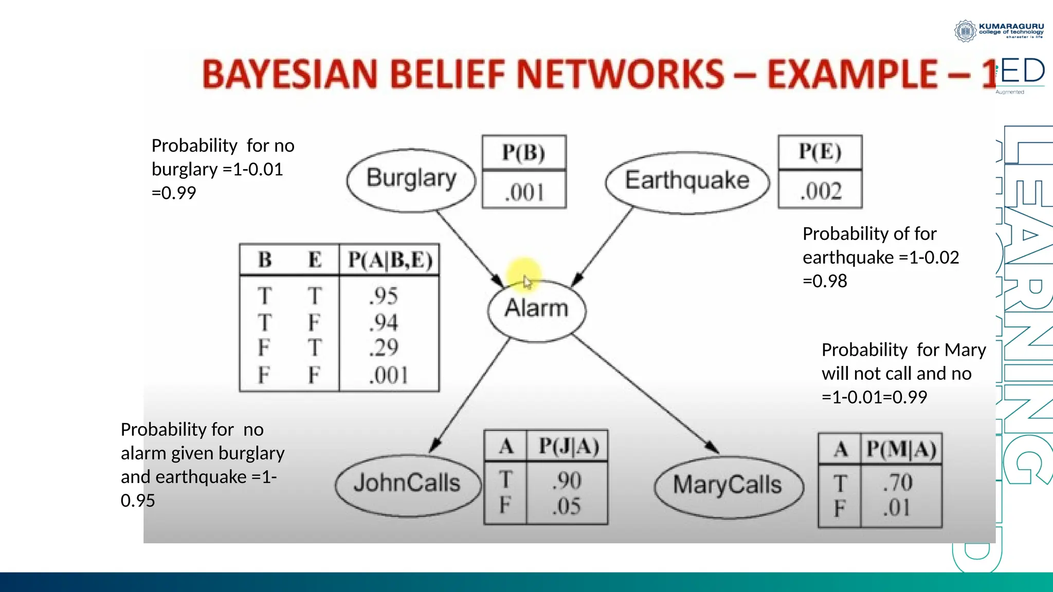
Probability for no burglary =1-0.01 =0.99 Probability of for earthquake =1-0.02 =0.98 Probability for no alarm given burglary and earthquake =1- 0.95 Probability for Mary will not call and no =1-0.01=0.99

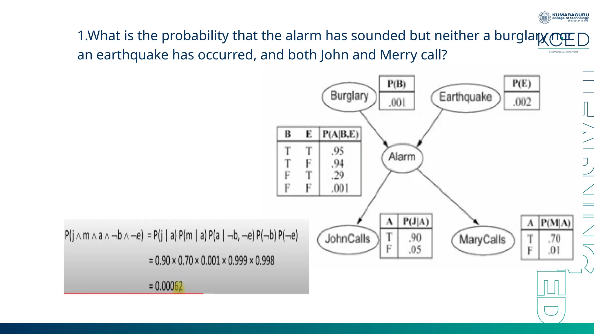
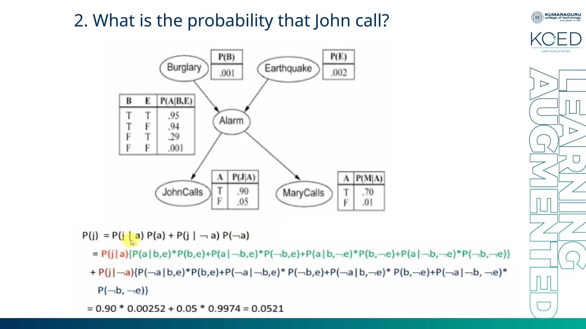
1.What is the probability that the alarm has sounded but neither a burglary nor an earthquake has occurred, and both John and Merry call?

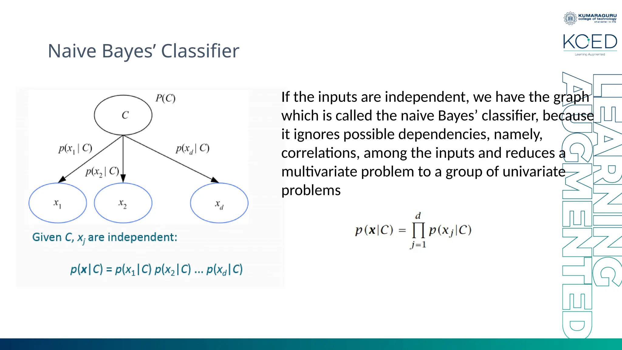
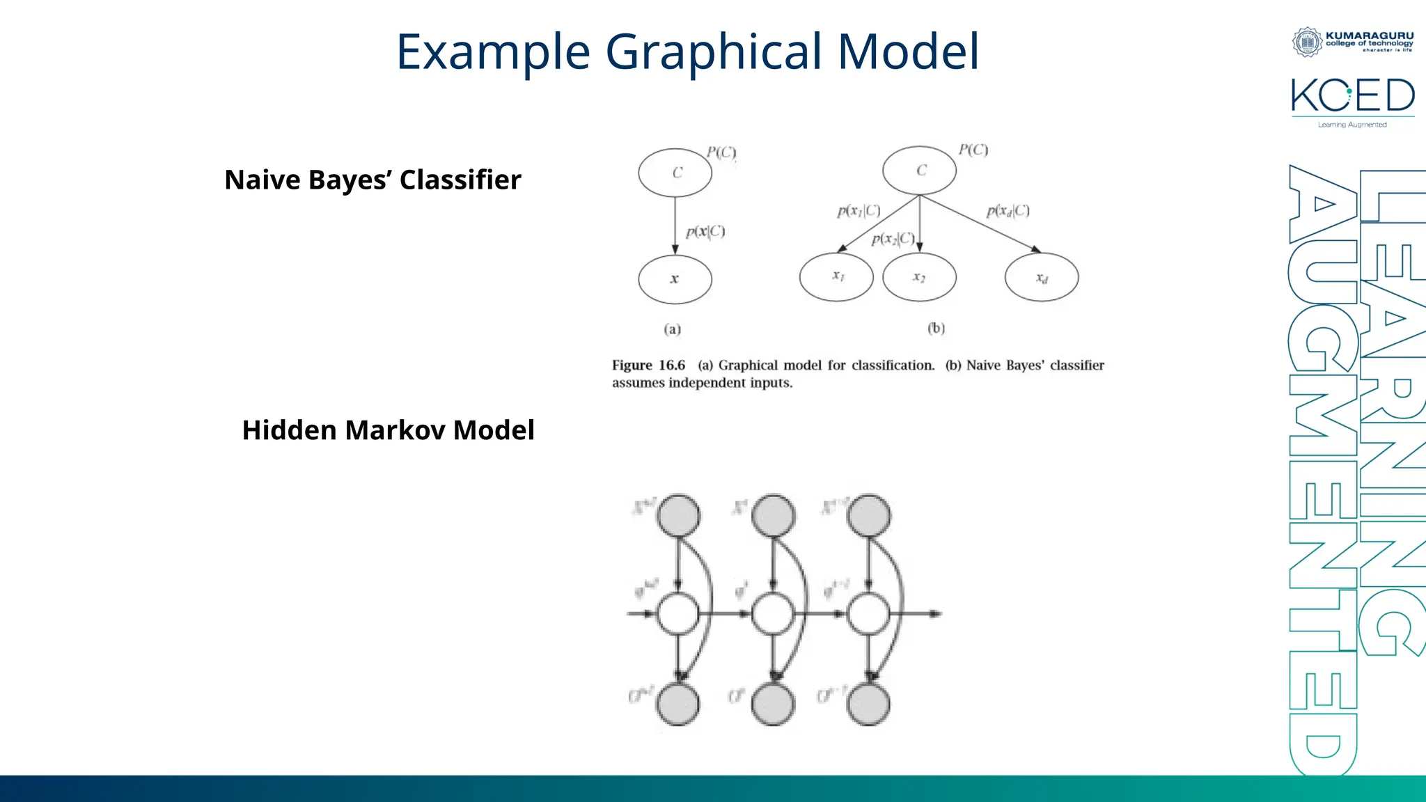
2. What is the probability that John call?

Naive Bayes’ Classifier If the inputs are independent, we have the graph which is called the naive Bayes’ classifier, because it ignores possible dependencies, namely, correlations, among the inputs and reduces a multivariate problem to a group of univariate problems

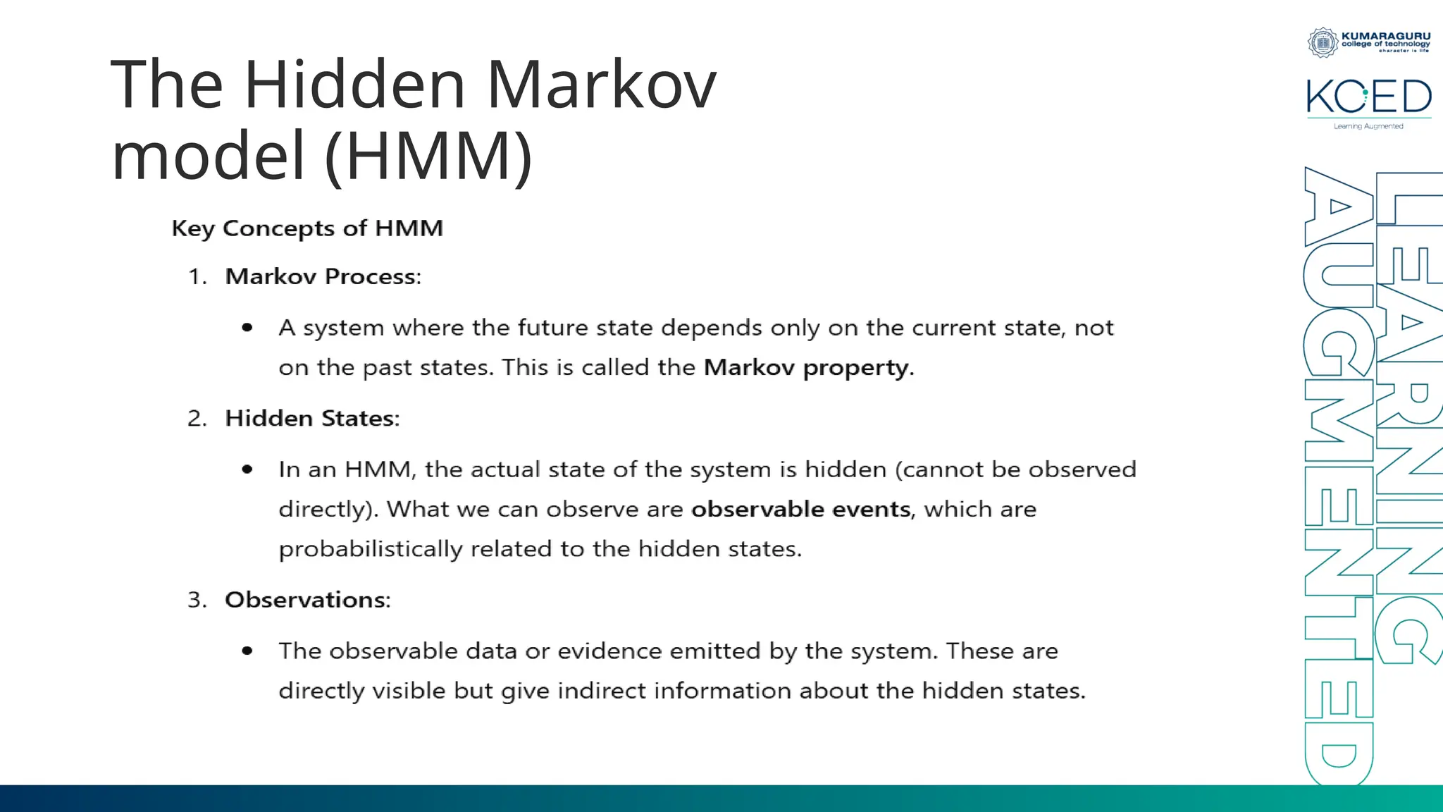
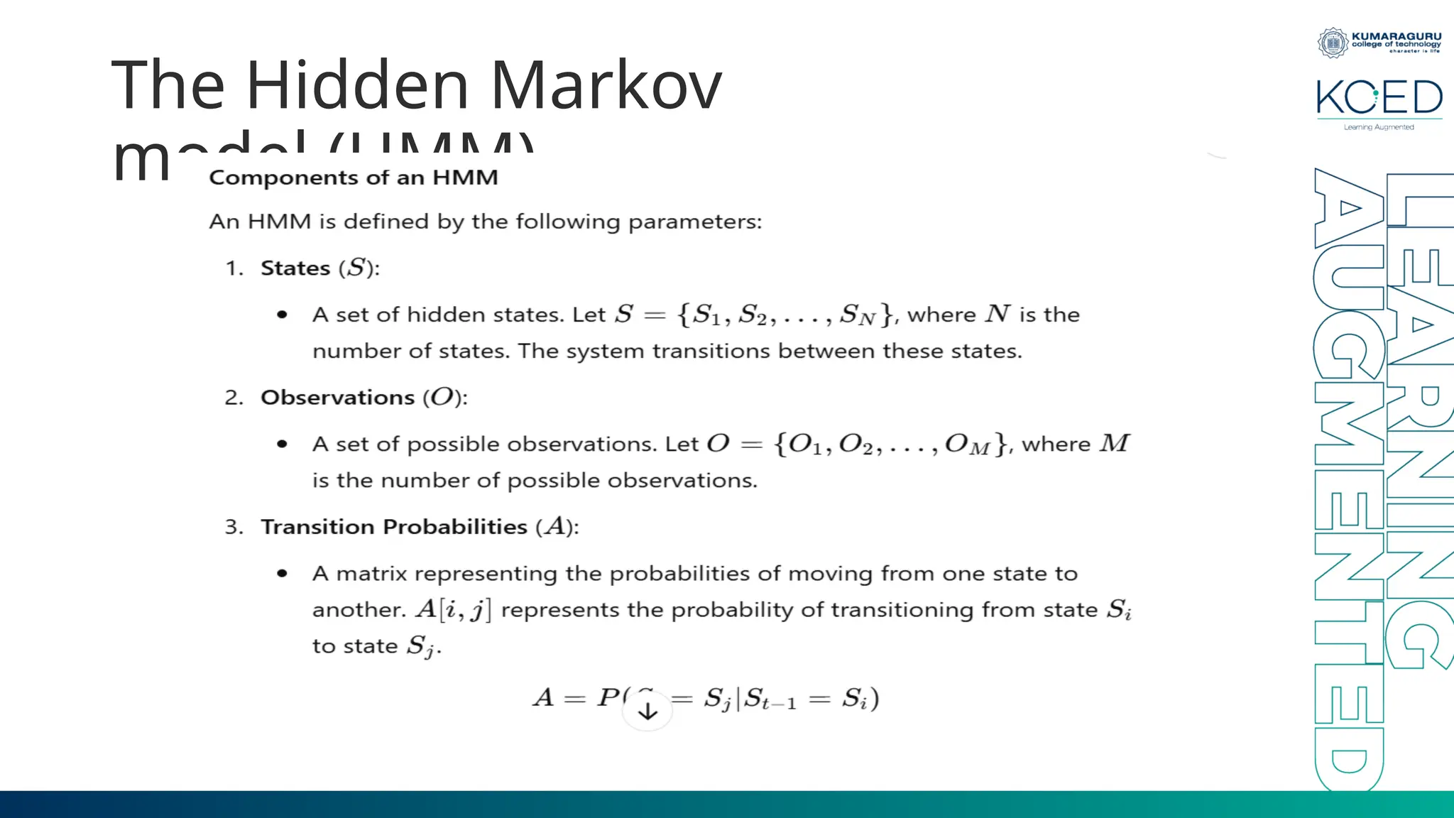
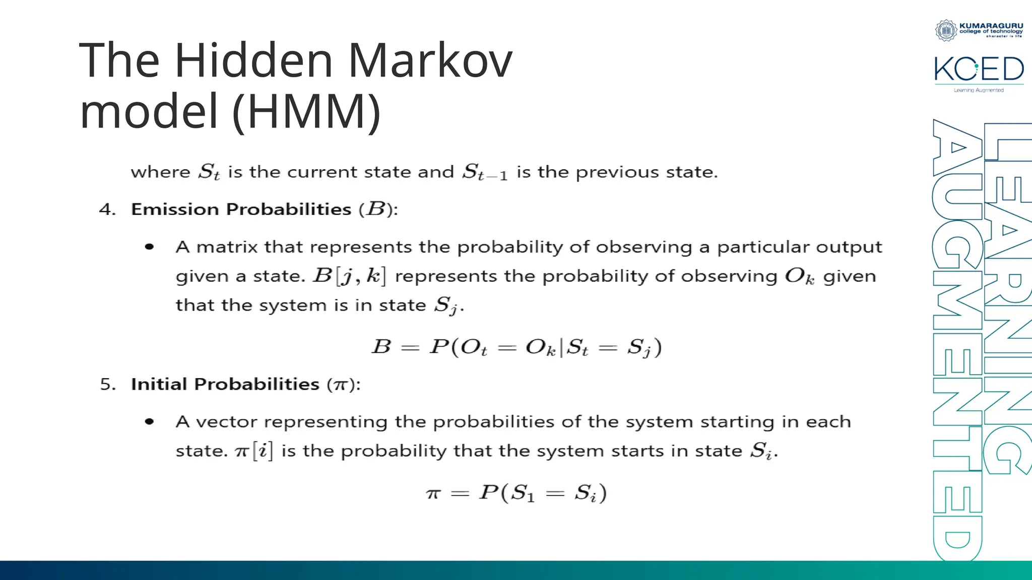
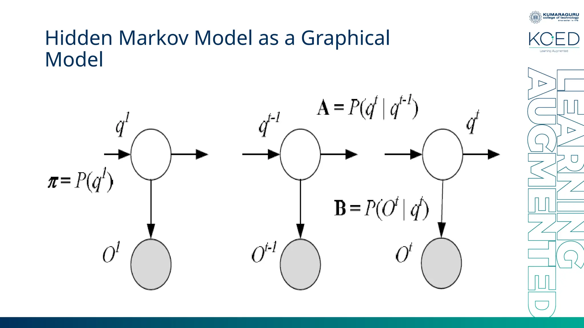
The Hidden Markov model (HMM) • The Hidden Markov model (HMM) is a statistical model and uses a Markov process that contains hidden and unknown parameters. • In this model, the observed parameters are used to identify the hidden parameters. These parameters are then used for further analysis • It is a probabilistic graphical model that is commonly used in statistical pattern recognition and classification.

Hidden Markov Model as a Graphical Model

Unit V -Graphical Models in artificial intelligence and machine learning

Unit V -Graphical Models in artificial intelligence and machine learning

More Related Content

Similar to Unit V -Graphical Models in artificial intelligence and machine learning

Recently uploaded

Unit V -Graphical Models in artificial intelligence and machine learning