Python as number crunching code glue

Python as number crunching glue Jiahao Chen jiahao@mit.edu @mitpostdoc theochem.mit.edu 1 Thursday, September 22, 2011

This is not a crash course on scientific computing or numerical linear algebra Recommended texts: nr.com 2 Thursday, September 22, 2011

NumPy and SciPy How to say: NumPy: no official pronunciation SciPy: “sigh pie” 3 Thursday, September 22, 2011

NumPy and SciPy How to say: NumPy: no official pronunciation SciPy: “sigh pie” Where to get: scipy.org, numpy.scipy.org You might already have it Otherwise, have fun installing it ;) 3 Thursday, September 22, 2011

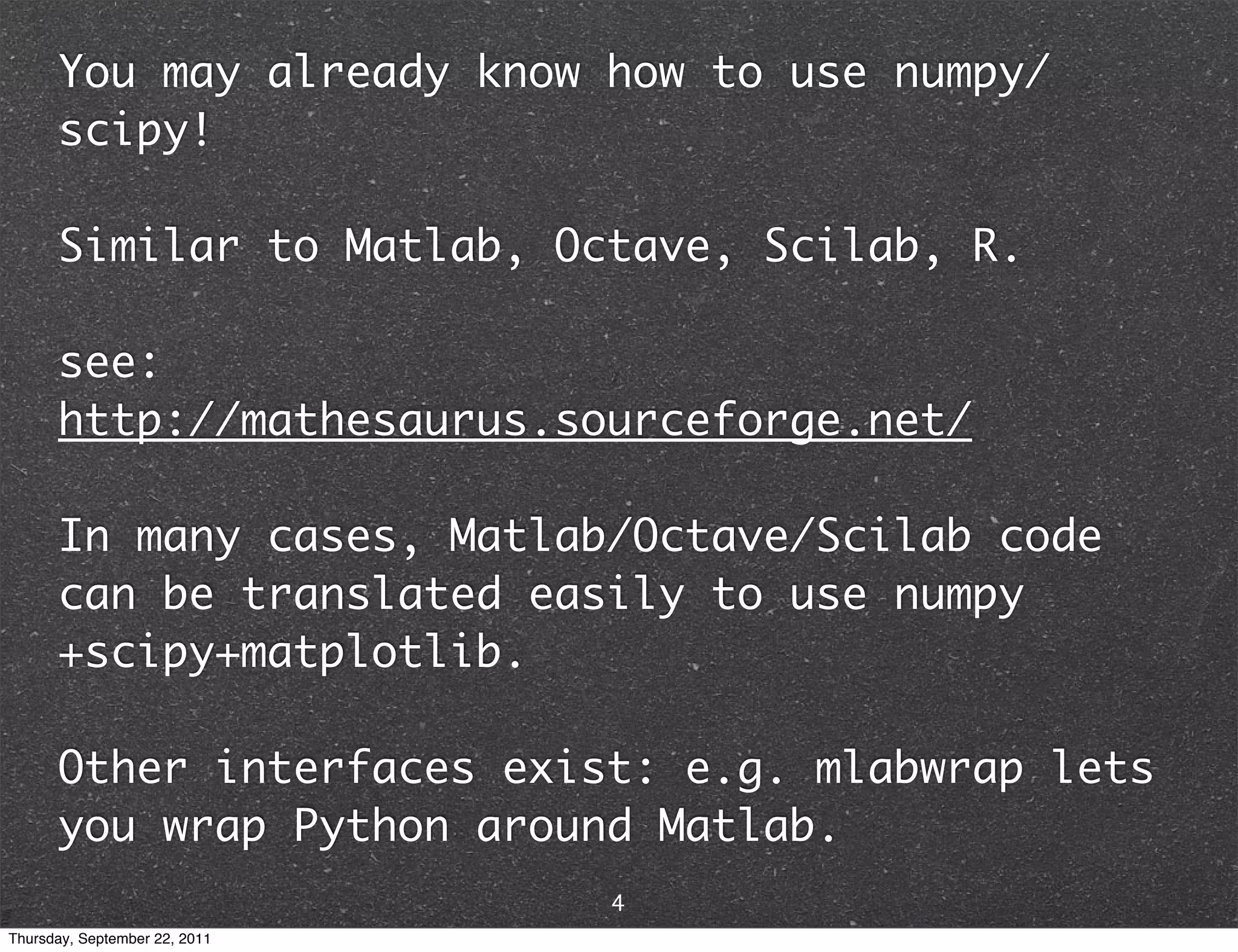
You may already know how to use numpy/ scipy! Similar to Matlab, Octave, Scilab, R. see: http://mathesaurus.sourceforge.net/ In many cases, Matlab/Octave/Scilab code can be translated easily to use numpy +scipy+matplotlib. Other interfaces exist: e.g. mlabwrap lets you wrap Python around Matlab. 4 Thursday, September 22, 2011

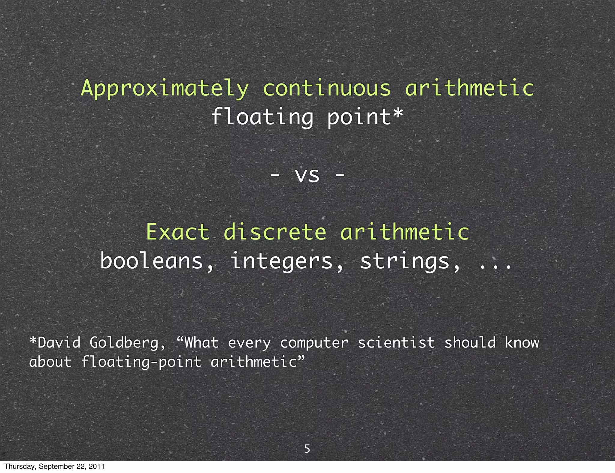
Approximately continuous arithmetic floating point* - vs - Exact discrete arithmetic booleans, integers, strings, ... *David Goldberg, “What every computer scientist should know about floating-point arithmetic” 5 Thursday, September 22, 2011

Using numpy can make code cleaner import numpy as np a = range(10000000) a = np.arange(10000000) b = range(10000000) b = np.arange(10000000) c = [] c = a + b for i in range(len(a)): c.append(a[i] + b[i]) What’s different?? 6 Thursday, September 22, 2011

What’s different?creates list of creates ndarray of dynamically typed int statically typed int import numpy as np a = range(10000000) a = np.arange(10000000) b = range(10000000) b = np.arange(10000000) c = [] #a+b is concatenation c = a + b #vectorized addition for i in range(len(a)): c.append(a[i] + b[i]) Using numpy can save lots of time 7.050s 0.333s (21x) a convenient interface to compiled C/Fortran libraries: BLAS, LAPACK, FFTW, UMFPACK,... 7 Thursday, September 22, 2011

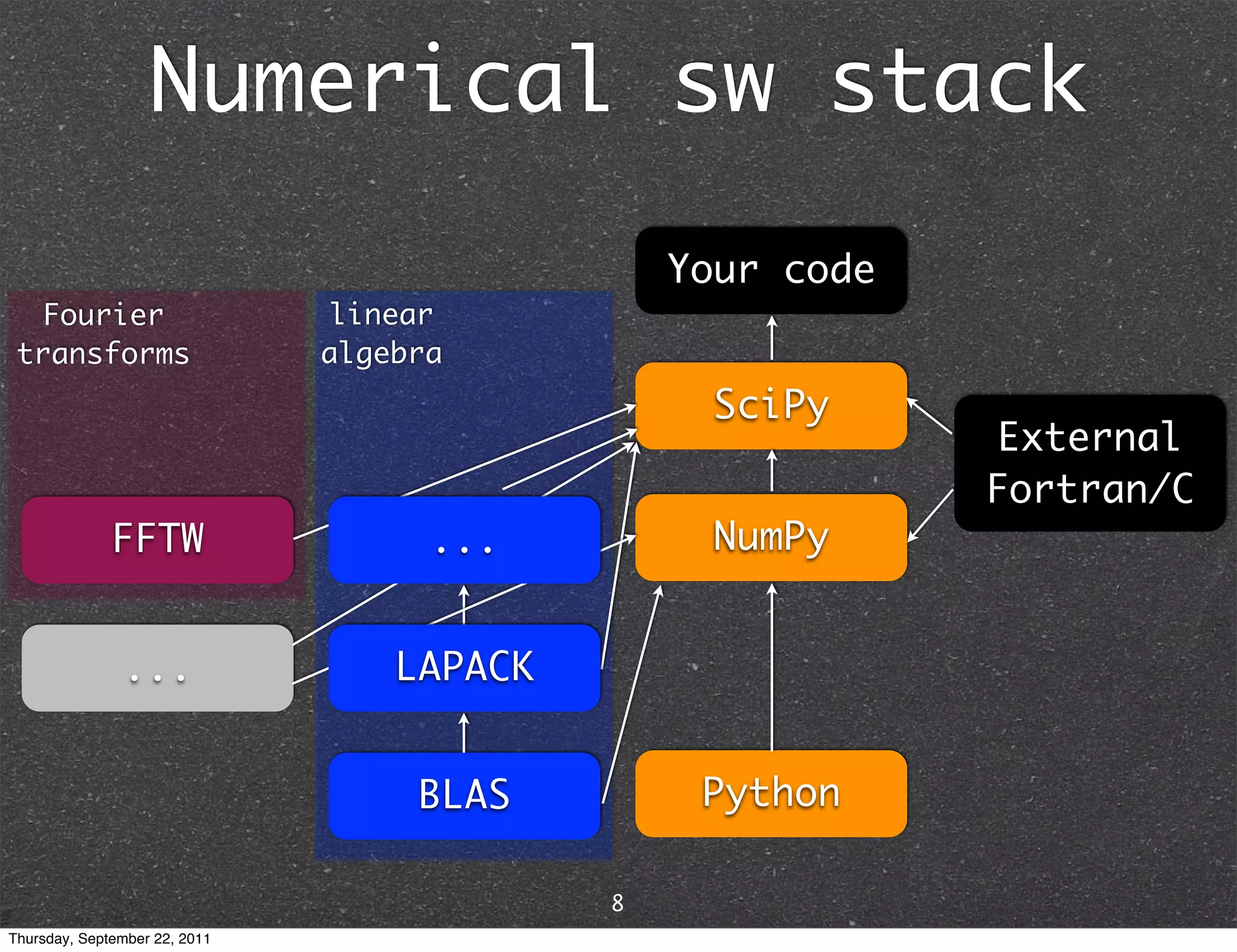
Numerical sw stack Your code Fourier linear transforms algebra SciPy External Fortran/C FFTW ... NumPy ... LAPACK BLAS Python 8 Thursday, September 22, 2011

“One thing that graduate students eventually learn is that you can hide just about anything in a NxN matrix... (for sufficiently large N)” - anonymous string theorist 9 Thursday, September 22, 2011

“One thing that graduate students eventually learn is that you can hide just about anything in a NxN matrix... (for sufficiently large N)” - anonymous string theorist If your data can be put into a matrix/vector, numpy/scipy can help you! 9 Thursday, September 22, 2011

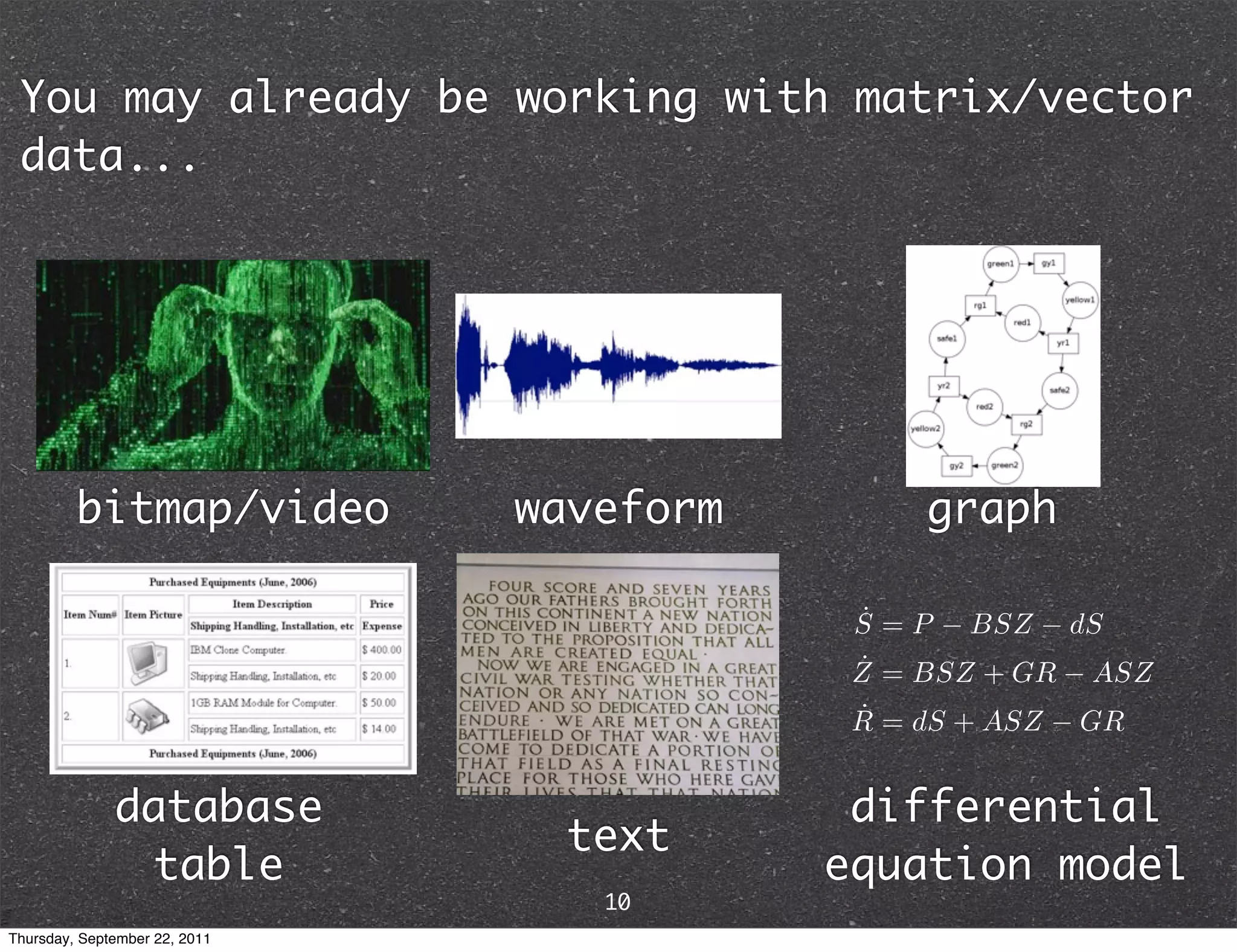
You may already be working with matrix/vector data... bitmap/video waveform graph database differential text table equation model 10 Thursday, September 22, 2011

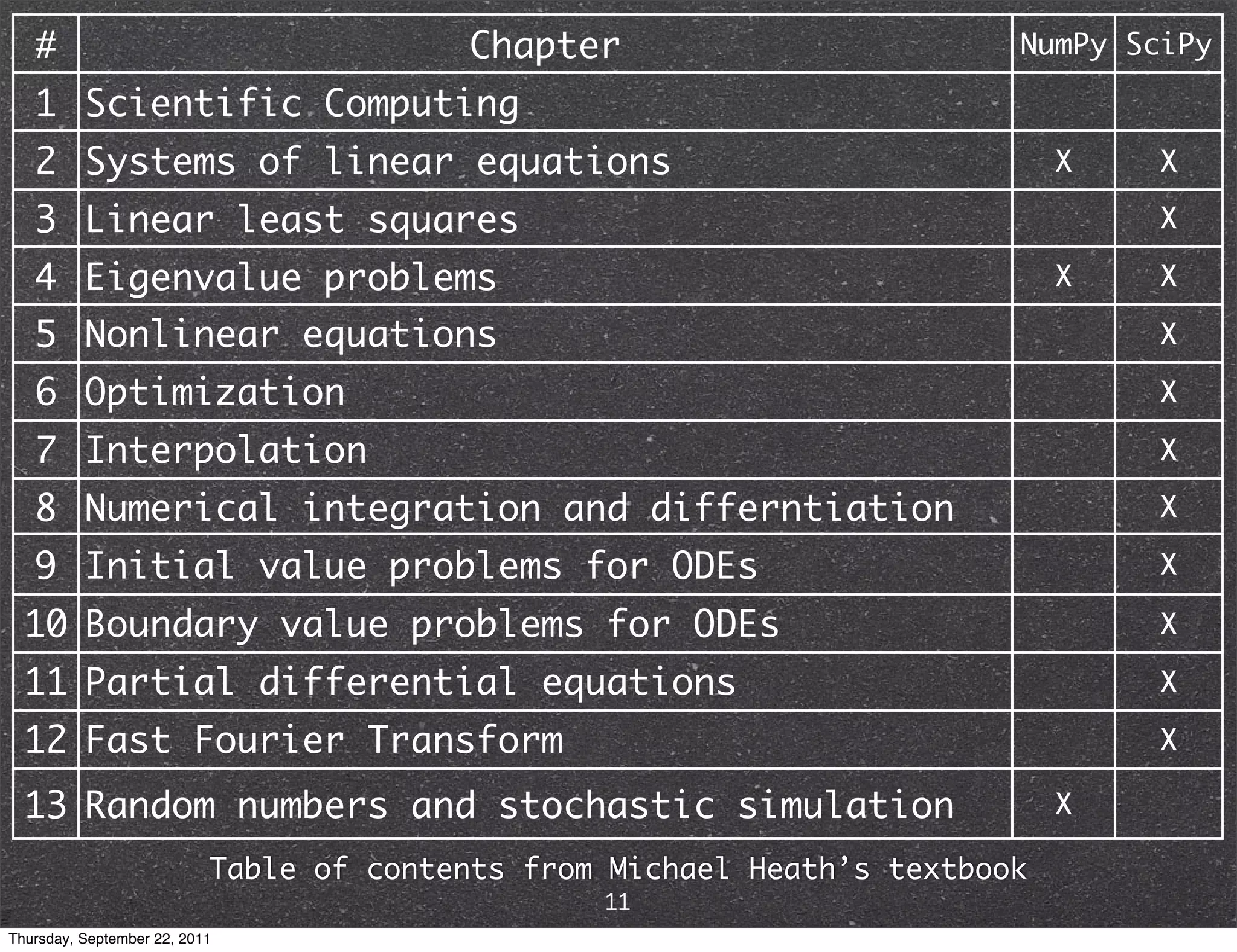
# Chapter NumPy SciPy 1 Scientific Computing 2 Systems of linear equations X X 3 Linear least squares X 4 Eigenvalue problems X X 5 Nonlinear equations X 6 Optimization X 7 Interpolation X 8 Numerical integration and differntiation X 9 Initial value problems for ODEs X 10 Boundary value problems for ODEs X 11 Partial differential equations X 12 Fast Fourier Transform X 13 Random numbers and stochastic simulation X Table of contents from Michael Heath’s textbook 11 Thursday, September 22, 2011

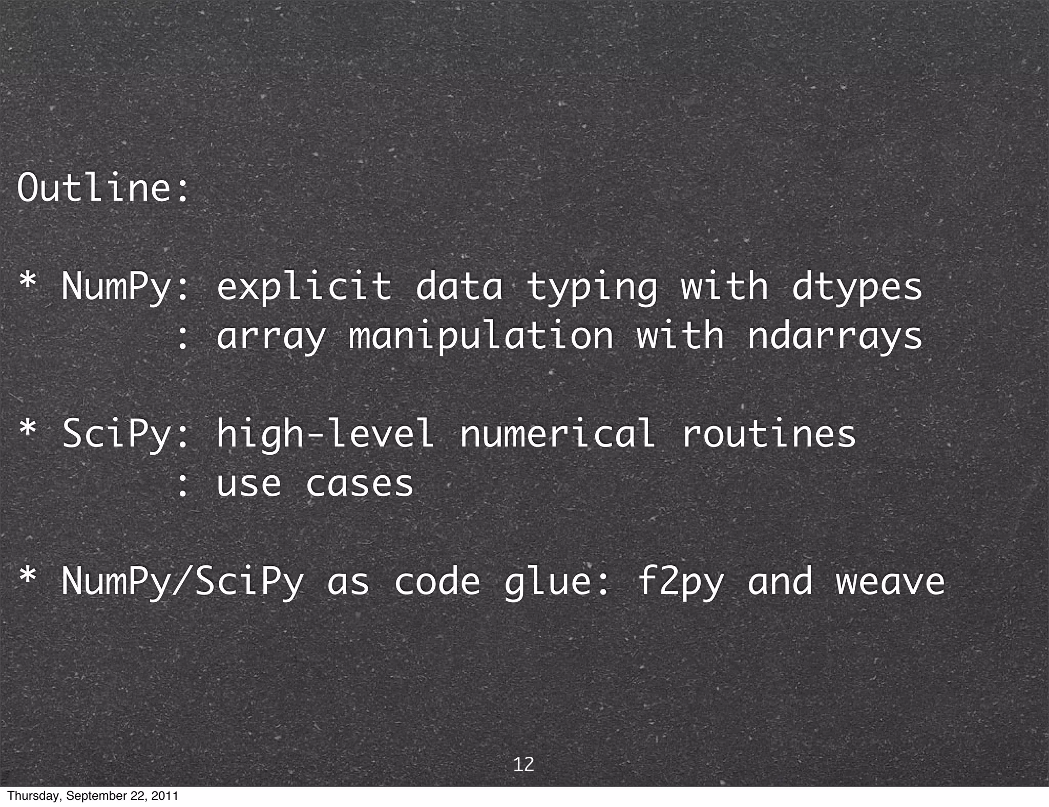
Outline: * NumPy: explicit data typing with dtypes : array manipulation with ndarrays * SciPy: high-level numerical routines : use cases * NumPy/SciPy as code glue: f2py and weave 12 Thursday, September 22, 2011

The most fundamental object in NumPy is the ndarray (N-dimensional array) v[:] vector M[:,:] matrix x[:,:,...,:] higher order tensor unlike built-in Python data types, ndarrays are designed for homogeneous, explicitly typed data 13 Thursday, September 22, 2011

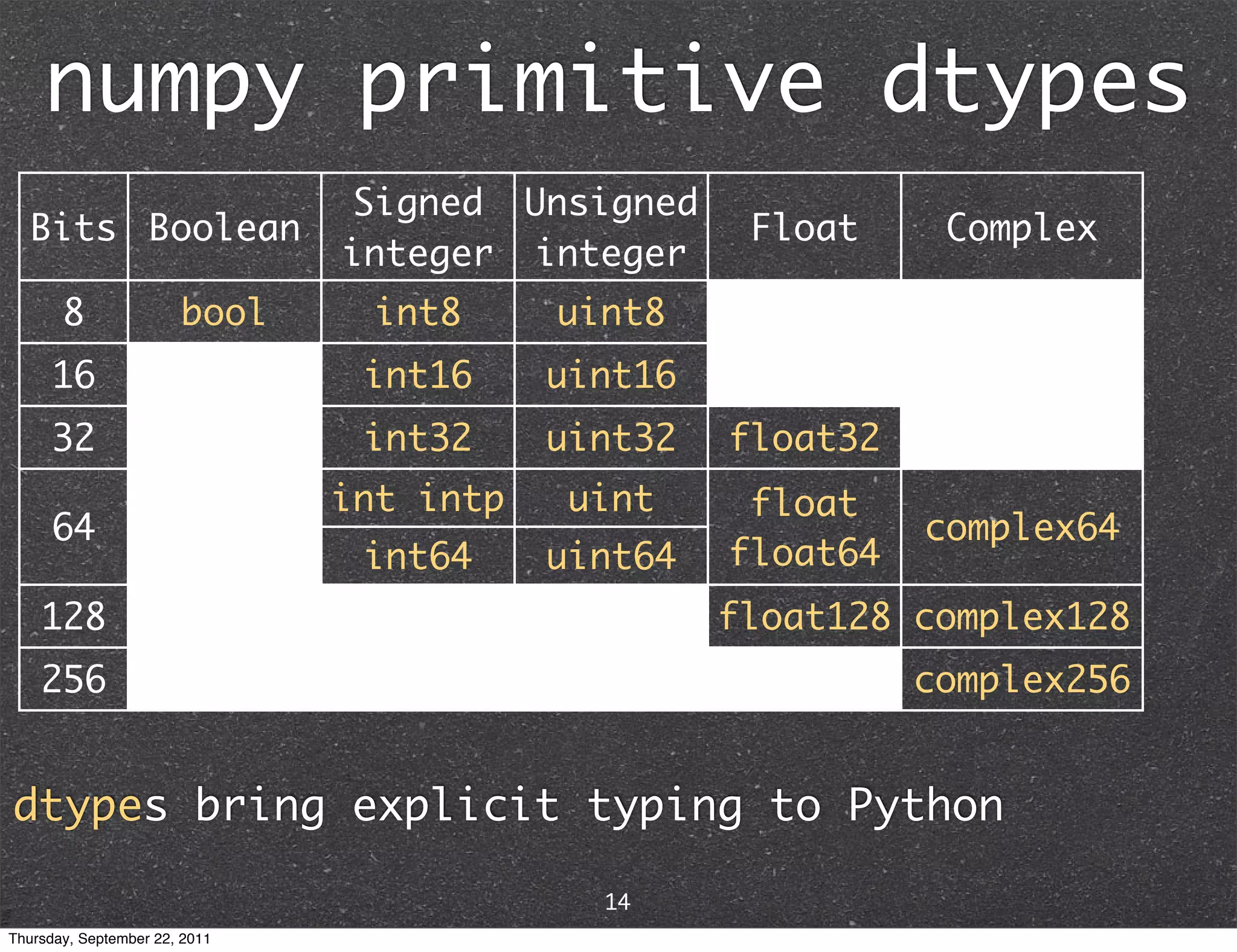
numpy primitive dtypes Signed Unsigned Bits Boolean Float Complex integer integer 8 bool int8 uint8 16 int16 uint16 32 int32 uint32 float32 int intp uint float 64 complex64 int64 uint64 float64 128 float128 complex128 256 complex256 dtypes bring explicit typing to Python 14 Thursday, September 22, 2011

Structured array: ndarray of data structure >>> mol = np.zeros(3, dtype=('uint8, 3float64')) >>> mol[0] = 8, (-0.464, 0.177, 0.0) >>> mol[1] = 1, (-0.464, 1.137, 0.0) >>> mol[2] = 1, (0.441, -0.143, 0.0) >>> mol array([(8, [-0.46400000000000002, 0.17699999999999999, 0.0]), (1, [-0.46400000000000002, 1.137, 0.0]), (1, [0.441, -0.14299999999999999, 0.0])], dtype=[('f0', '|u1'), ('f1', '<f8', (3,))]) Recarray: ndarray of data structure with named fields (record) >>> mol = np.array(mol, dtype={'atomicnum':('uint8',0), 'coords':('3float64',1)}) >>> mol['atomicnum'] array([8, 1, 1], dtype=uint8) 15 Thursday, September 22, 2011

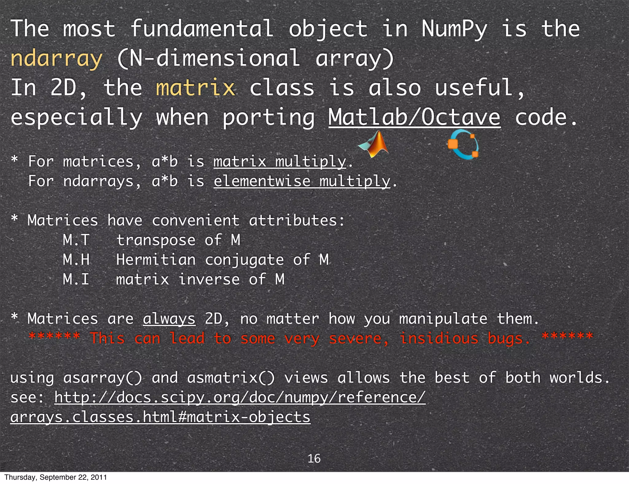
The most fundamental object in NumPy is the ndarray (N-dimensional array) In 2D, the matrix class is also useful, especially when porting Matlab/Octave code. * For matrices, a*b is matrix multiply. For ndarrays, a*b is elementwise multiply. * Matrices have convenient attributes: M.T transpose of M M.H Hermitian conjugate of M M.I matrix inverse of M * Matrices are always 2D, no matter how you manipulate them. ****** This can lead to some very severe, insidious bugs. ****** using asarray() and asmatrix() views allows the best of both worlds. see: http://docs.scipy.org/doc/numpy/reference/ arrays.classes.html#matrix-objects 16 Thursday, September 22, 2011

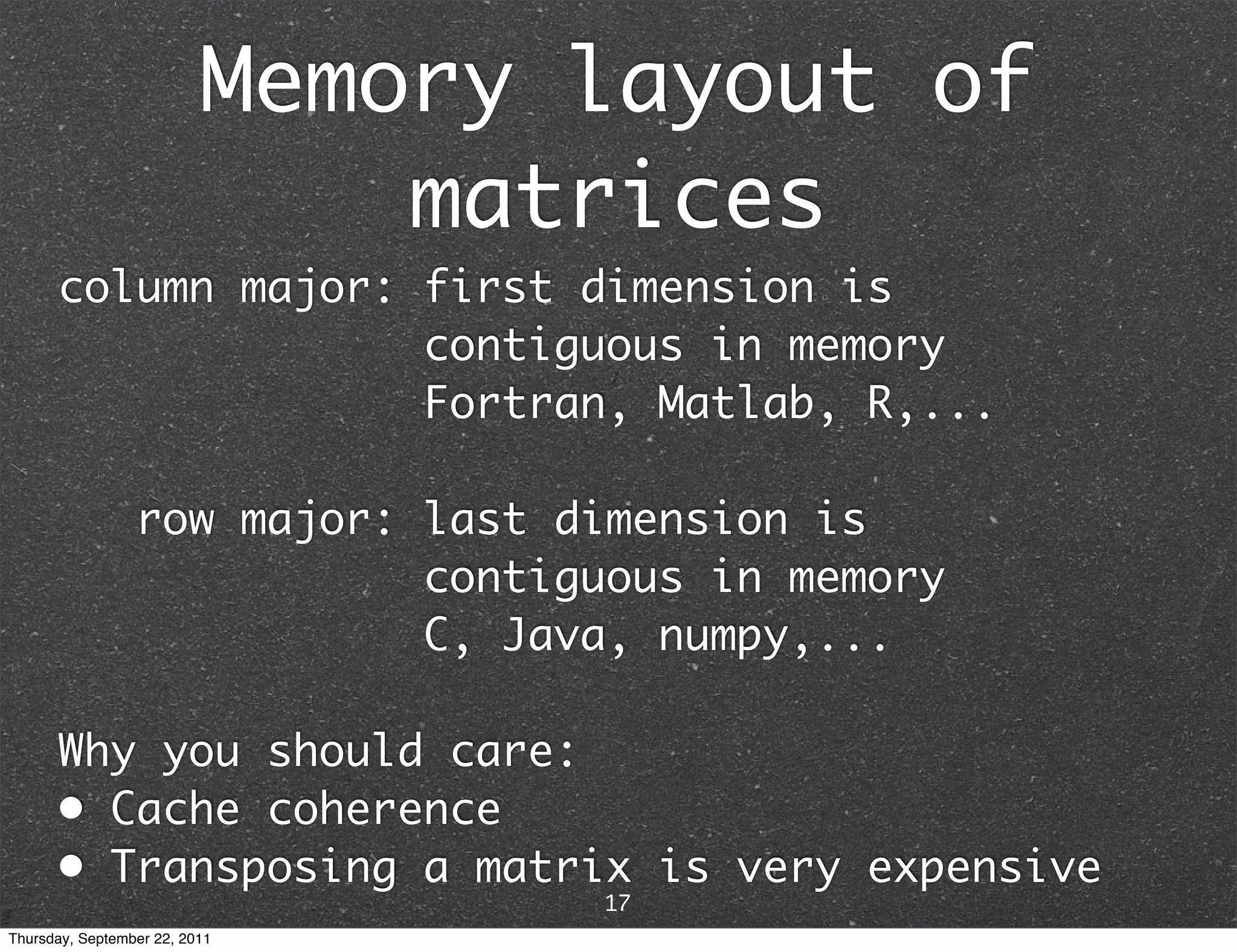
Memory layout of matrices column major: first dimension is contiguous in memory Fortran, Matlab, R,... row major: last dimension is contiguous in memory C, Java, numpy,... Why you should care: • Cache coherence • Transposing a matrix is very expensive 17 Thursday, September 22, 2011

Creating ndarrays • from Python iterable: lists, tuples,... e.g. array([1, 2, 3]) == asarray((1, 2, 3)) • from intrinsic functions empty() allocates memory only zeros() initializes to 0 ones() initializes to 1 arange() creates a uniform range rand() initializes to uniform random randn() initializes to standard normal random ... • from binary representation in string/buffer • from file on disk 18 Thursday, September 22, 2011

Generating ndarrays fromfunction() creates an ndarray whose entries are functions of its indices e.g. the Hilbert matrix 1..n >>> np.fromfunction(lambda i,j: 1./(i+j+1), (4,4)) array([[ 1. , 0.5 , 0.33333333, 0.25 ], [ 0.5 , 0.33333333, 0.25 , 0.2 ], [ 0.33333333, 0.25 , 0.2 , 0.16666667], [ 0.25 , 0.2 , 0.16666667, 0.14285714]]) 19 Thursday, September 22, 2011

Generating ndarrays arange(): like range() but accepts floats >>> import numpy as np >>> np.arange(2, 2.5, 0.1) array([ 2. , 2.1, 2.2, 2.3, 2.4]) linspace(): creates array with speciﬁed number of elements, spaced equally between the speciﬁed beginning and ending. >>> np.linspace(2.0, 2.4, 5) array([ 2. , 2.1, 2.2, 2.3, 2.4]) 20 Thursday, September 22, 2011

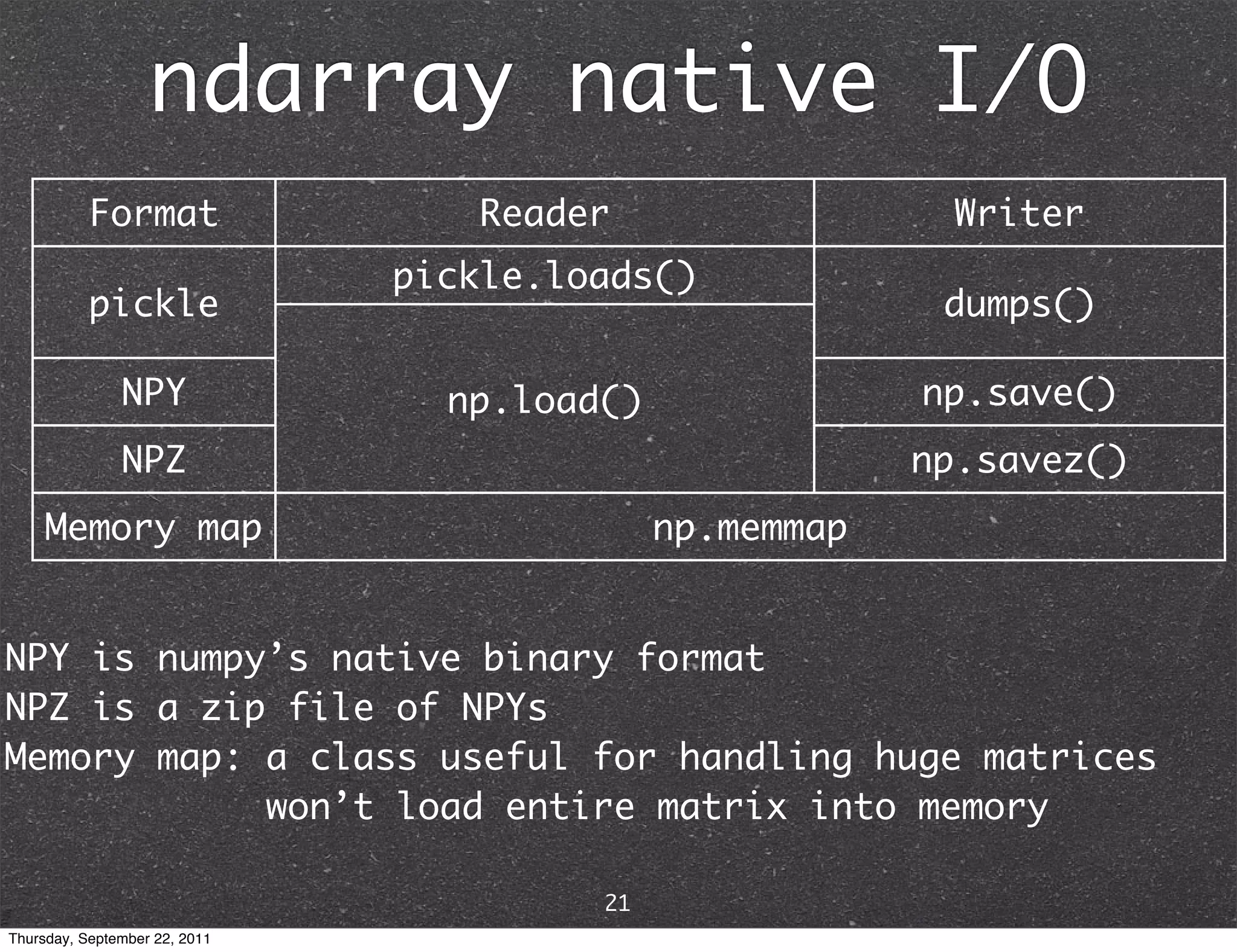
ndarray native I/O Format Reader Writer pickle.loads() pickle dumps() NPY np.load() np.save() NPZ np.savez() Memory map np.memmap NPY is numpy’s native binary format NPZ is a zip file of NPYs Memory map: a class useful for handling huge matrices won’t load entire matrix into memory 21 Thursday, September 22, 2011

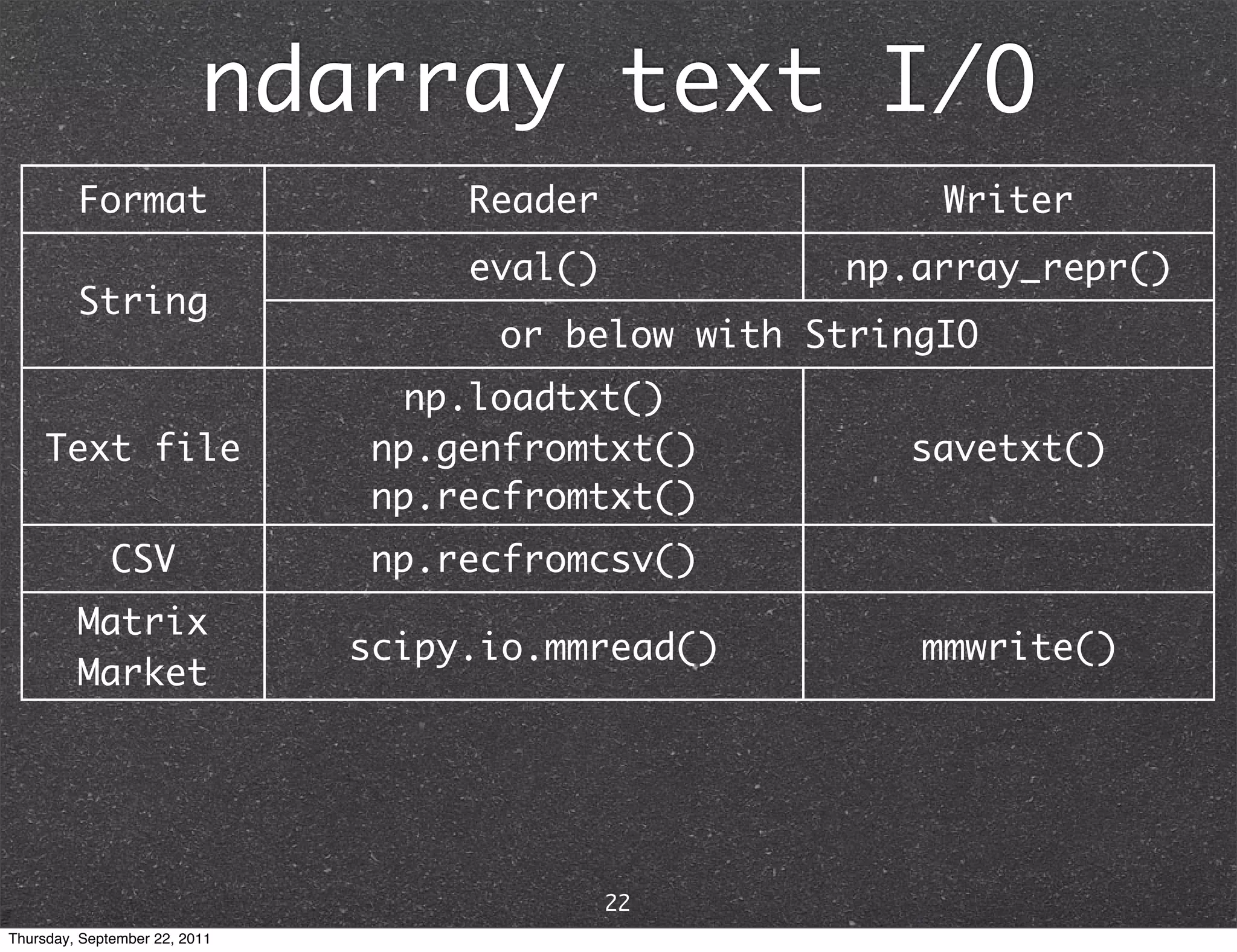
ndarray text I/O Format Reader Writer eval() np.array_repr() String or below with StringIO np.loadtxt() Text file np.genfromtxt() savetxt() np.recfromtxt() CSV np.recfromcsv() Matrix scipy.io.mmread() mmwrite() Market 22 Thursday, September 22, 2011

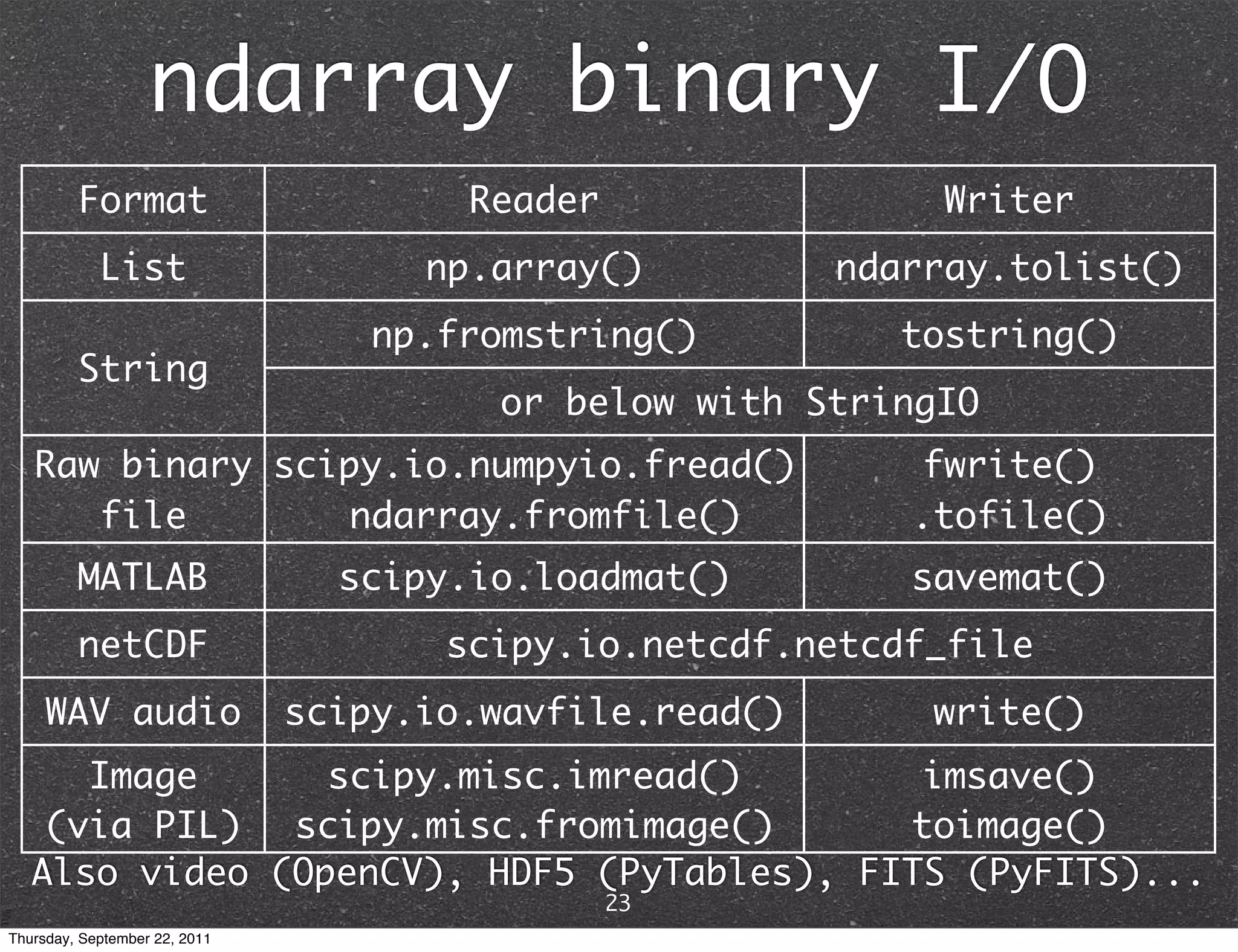
ndarray binary I/O Format Reader Writer List np.array() ndarray.tolist() np.fromstring() tostring() String or below with StringIO Raw binary scipy.io.numpyio.fread() fwrite() file ndarray.fromfile() .tofile() MATLAB scipy.io.loadmat() savemat() netCDF scipy.io.netcdf.netcdf_file WAV audio scipy.io.wavfile.read() write() Image scipy.misc.imread() imsave() (via PIL) scipy.misc.fromimage() toimage() Also video (OpenCV), HDF5 (PyTables), FITS (PyFITS)... 23 Thursday, September 22, 2011

Indexing >>> x = np.arange(12).reshape(3,4); x array([[ 0, 1, 2, 3], [ 4, 5, 6, 7], [ 8, 9, 10, 11]]) >>> x[1,2] 6 >>> x[2,-1] row, then column 11 >>> x[0][2] 2 >>> x[(2,2)] #tuple 10 >>> x[:1] #slices return views, not copies array([[0, 1, 2, 3]]) >>> x[::2,1:4:2] array([[ 1, 3], [ 9, 11]]) 24 Thursday, September 22, 2011

Fancy indexing >>> x = np.arange(12).reshape(3,4); x array([[ 0, 1, 2, 3], [ 4, 5, 6, 7], [ 8, 9, 10, 11]]) >>> x[(2,2)] array index 10 >>> x[np.array([2,2])] #same as x[[2,2]] array([[ 8, 9, 10, 11], [ 8, 9, 10, 11]]) >>> x[np.array([1,0]), np.array([2,1])] array([6, 1]) >>> x[x>8] Boolean mask array([ 9, 10, 11]) >>> x>8 array([[False, False, False, False], [False, False, False, False], [False, True, True, True]], dtype=bool) 25 Thursday, September 22, 2011

Fancy indexing II >>> y = np.arange(1*2*3*4).reshape(1,2,3,4); y array([[[[ 0, 1, 2, 3], [ 4, 5, 6, 7], [ 8, 9, 10, 11]], [[12, 13, 14, 15], [16, 17, 18, 19], [20, 21, 22, 23]]]]) >>> y[0, Ellipsis, 0] # == y[0, ..., 0] == [0,:,:,0] array([[ 0, 4, 8], [12, 16, 20]]) >>> y[0, 0, 0, slice(2,4)] # == y[(0, 0, 0, 2:4)] array([2, 3]) 26 Thursday, September 22, 2011

Broadcasting What happens when you multiply ndarrays of different dimensions? Case I: trailing dimensions match >>> x #.shape = (3,4) array([[ 0, 1, 2, 3], >>> y * x [ 4, 5, 6, 7], array([[[[ 0, 1, 4, 9], [ 8, 9, 10, 11]]) [ 16, 25, 36, 49], >>> y #.shape = (1,2,3,4) [ 64, 81, 100, 121]], array([[[[ 0, 1, 2, 3], [ 4, 5, 6, 7], [[ 0, 13, 28, 45], [ 8, 9, 10, 11]], [ 64, 85, 108, 133], [160, 189, 220, 253]]]]) [[12, 13, 14, 15], [16, 17, 18, 19], [20, 21, 22, 23]]]]) 27 Thursday, September 22, 2011

Broadcasting What happens when you multiply ndarrays of different dimensions? Case II: trailing dimension is 1 >>> b.shape = 4,1 >>> a + b >>> a = np.arange(4); a array([[3, 4, 5, 6], array([0, 1, 2, 3]) [2, 3, 4, 5], >>> b = np.arange(4)[::-1]; b [1, 2, 3, 4], array([3, 2, 1, 0]) [0, 1, 2, 3]]) >>> a + b array([3, 3, 3, 3]) >>> b.shape = 1,4 >>> a + b array([[3, 3, 3, 3]]) 28 Thursday, September 22, 2011

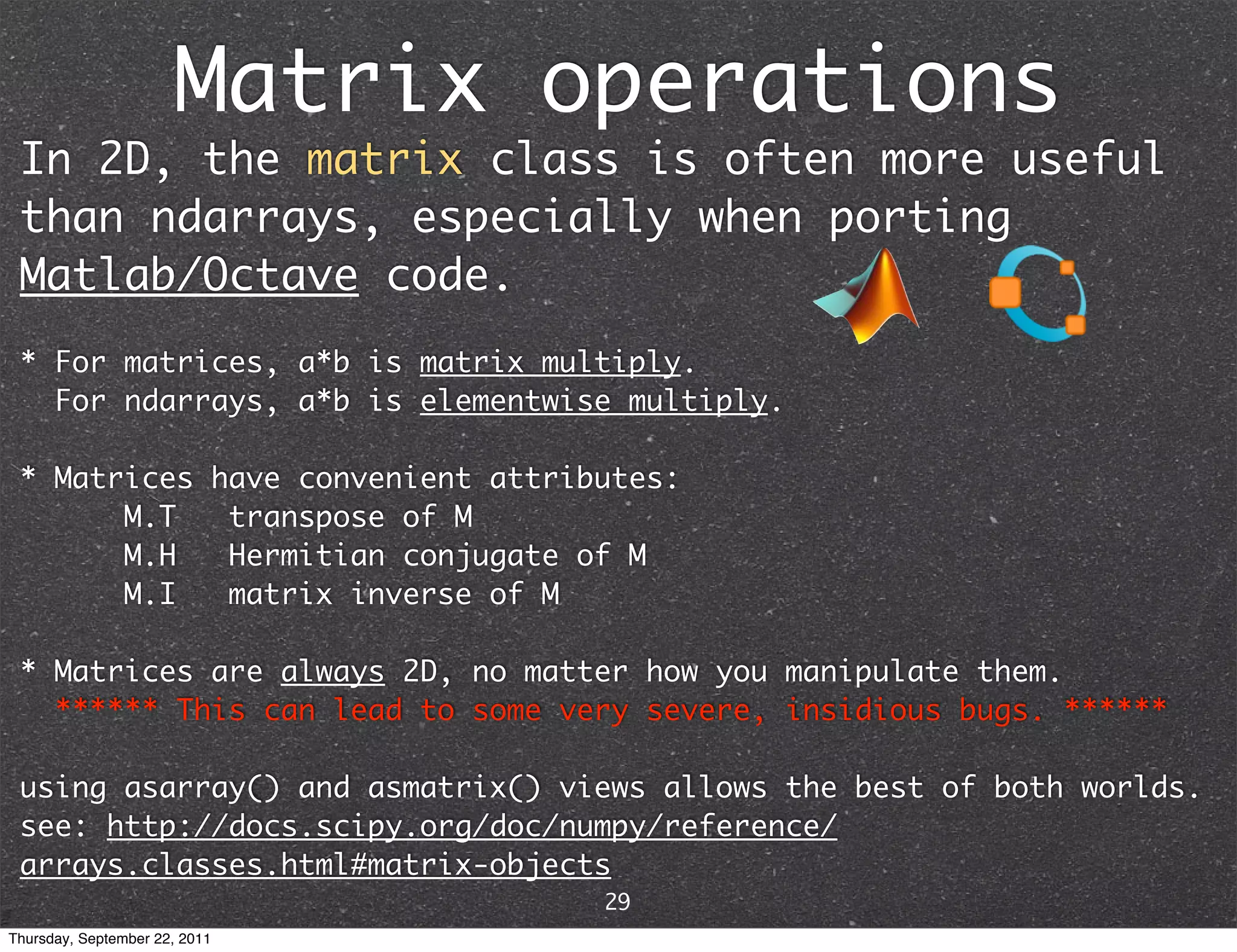
Matrix operations In 2D, the matrix class is often more useful than ndarrays, especially when porting Matlab/Octave code. * For matrices, a*b is matrix multiply. For ndarrays, a*b is elementwise multiply. * Matrices have convenient attributes: M.T transpose of M M.H Hermitian conjugate of M M.I matrix inverse of M * Matrices are always 2D, no matter how you manipulate them. ****** This can lead to some very severe, insidious bugs. ****** using asarray() and asmatrix() views allows the best of both worlds. see: http://docs.scipy.org/doc/numpy/reference/ arrays.classes.html#matrix-objects 29 Thursday, September 22, 2011

Matrix functions You can apply a function elementwise to a matrix... >>> from numpy import array, exp >>> X = array([[1, 1], [1, 0]]) >>> exp(X) array([[ 2.71828183, 2.71828183], [ 2.71828183, 1.]]) ...or a matrix version of that function >>> from scipy.linalg import expm >>> expm(X) array([[ 2.71828183, 7.3890561 ], [ 1. , 2.71828183]]) other functions in scipy.linalg.matfuncs 30 Thursday, September 22, 2011

SciPy by example * Data fitting * Signal matching * Disease outbreak modeling (epidemiology) http://scipy-central.org/ 31 Thursday, September 22, 2011

Least-squares curve fitting from scipy import * fit data to model from scipy.optimize import leastsq from matplotlib.pyplot import plot #Make up data x(t) with Gaussian noise num_points = 150 t = linspace(5, 8, num_points) x = 11.86*cos(2*pi/0.81*t-1.32) + 0.64*t +4*((0.5-rand(num_points))* exp(2*rand(num_points)**2)) # Target function model = lambda p, x: p[0]*cos(2*pi/p[1]*x+p[2]) + p[3]*x # Distance to the target function error = lambda p, x, y: model(p, x) - y # Initial guess for the parameters p0 = [-15., 0.8, 0., -1.] p1, _ = leastsq(error, p0, args=(t, x)) t2 = linspace(t.min(), t.max(), 100) plot(t, x, "ro", t2, model(p1, t2), "b-") raw_input() 32 Thursday, September 22, 2011

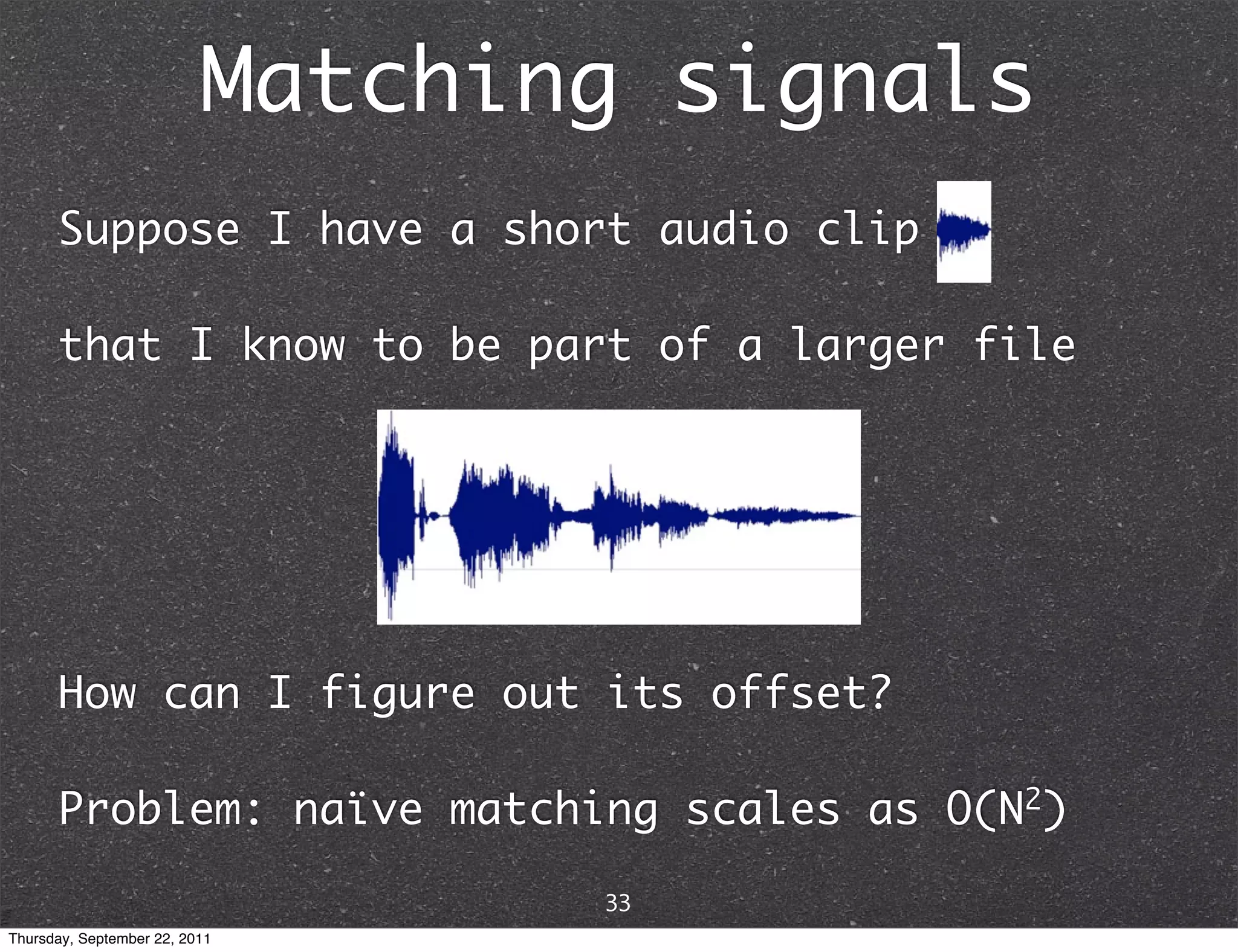
Matching signals Suppose I have a short audio clip that I know to be part of a larger file How can I figure out its offset? Problem: naïve matching scales as O(N2) 33 Thursday, September 22, 2011

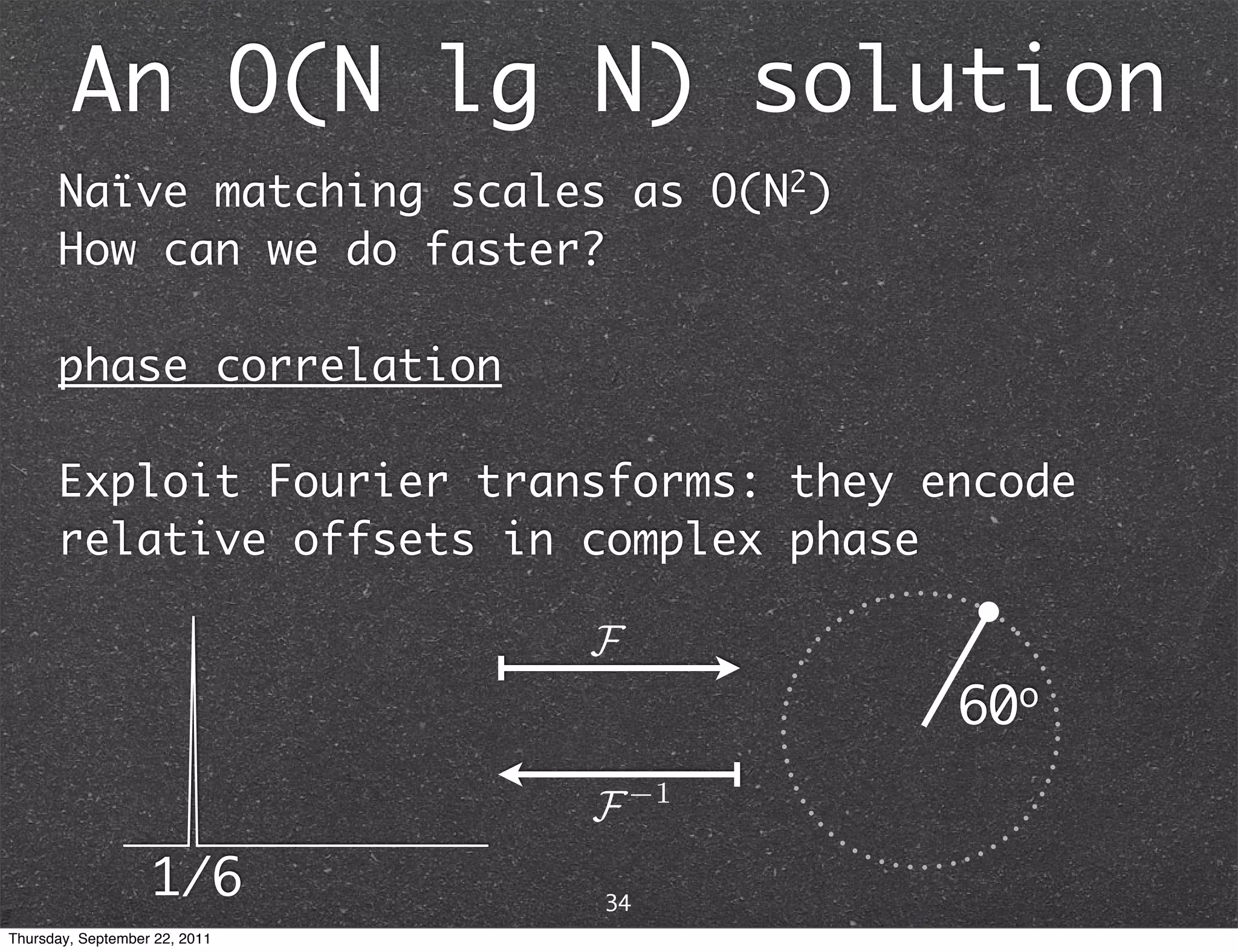
An O(N lg N) solution Naïve matching scales as O(N2) How can we do faster? phase correlation Exploit Fourier transforms: they encode relative offsets in complex phase 60o 1/6 34 Thursday, September 22, 2011

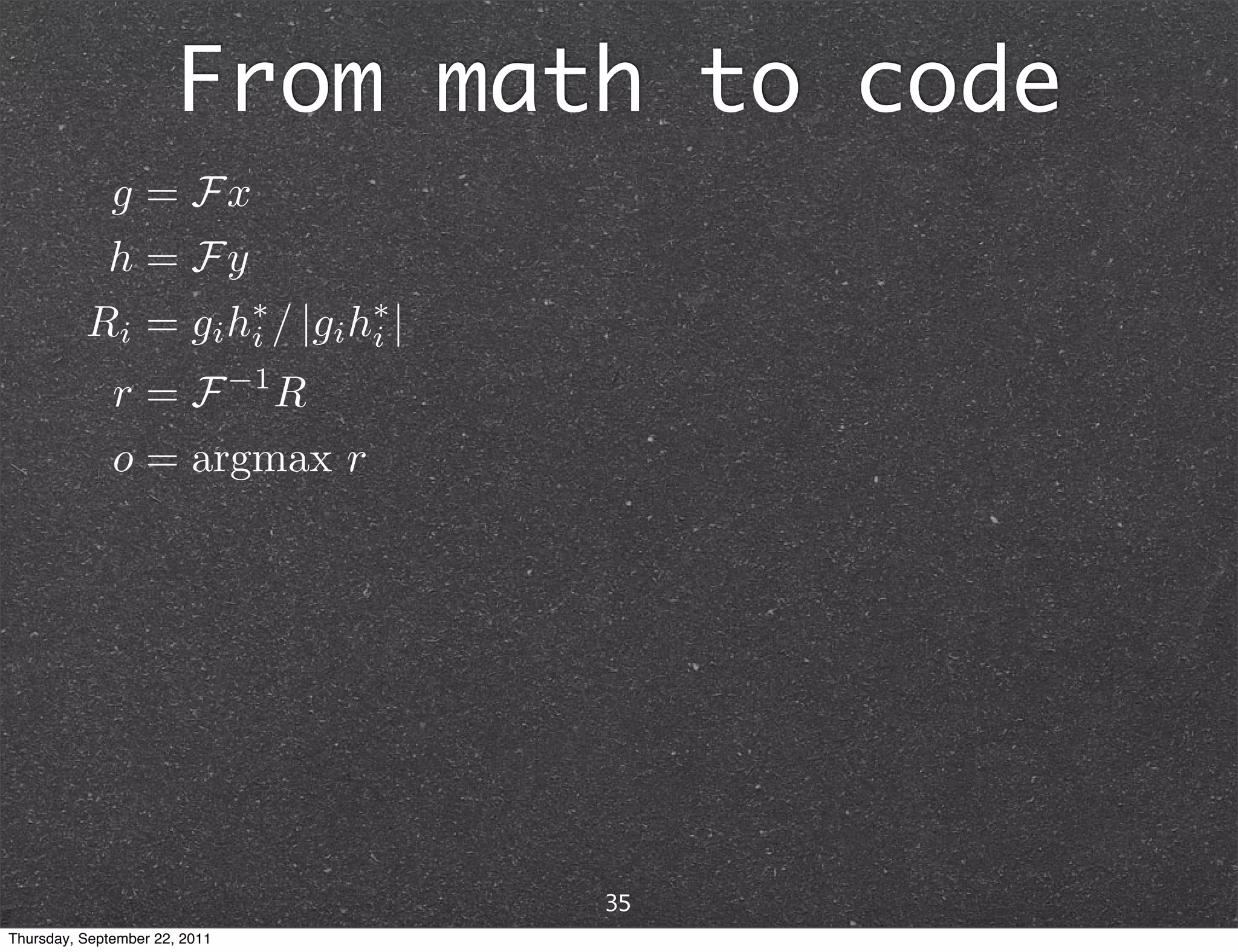
From math to code 35 Thursday, September 22, 2011

From math to code import numpy #Make up some data N = 30000 idx = 24700 size = 300 data = numpy.random.rand(N) frag_pad = numpy.zeros(N) frag = data[idx:idx+size] frag_pad[:size] = frag #Compute phase correlation data_ft = numpy.fft.rfft(data) frag_ft = numpy.fft.rfft(frag_pad) phase = data_ft * numpy.conj(frag_ft) phase /= abs(phase) cross_correlation = numpy.fft.irfft(phase) offset = numpy.argmax(cross_correlation) print 'Input offset: %d, computed: %d' % (idx, offset) from matplotlib.pyplot import plot plot(cross_correlation) raw_input() #Pause 35 Thursday, September 22, 2011

Modeling a zombie apocalypse http://blogs.cdc.gov/publichealthmatters/2011/05/preparedness-101- zombie-apocalypse/ 36 Thursday, September 22, 2011

Modeling a zombie apocalypse Each person can be in one of three states Normal (S) Zombie Dead (R) http://www.scipy.org/Cookbook/Zombie_Apocalypse_ODEINT 37 Thursday, September 22, 2011

Modeling a zombie apocalypse transmission (B) resurrection (G) Normal (S) Zombie Dead (R) + destruction (A) birth (P) normal death Various processes connect these states http://www.scipy.org/Cookbook/Zombie_Apocalypse_ODEINT 38 Thursday, September 22, 2011

From math to code B G from numpy import linspace from scipy.integrate import odeint P = 0 # birth rate d = 0.0001 # natural death rate S Z R B = 0.0095 # transmission rate + A G = 0.0001 # resurrection rate A = 0.0001 # destruction rate r d def f(y, t): Si, Zi, Ri = y return [P - B*Si*Zi - d*Si, B*Si*Zi + G*Ri - A*Si*Zi, d*Si + A*Si*Zi - G*Ri] y0 = [500, 0, 0] # initial conditions t = linspace(0, 5., 1000) # time grid soln = odeint(f, y0, t) # solve ODE S, Z, R = soln[:, :].T http://www.scipy.org/Cookbook/Zombie_Apocalypse_ODEINT 39 Thursday, September 22, 2011

Using external code “NumPy can get you most of the way to compiled speeds through vectorization. In situations where you still need the last ounce of speed in a critical section, or when it either requires a PhD in NumPy-ology to vectorize the solution or it results in too much memory overhead, you can reach for Cython or Weave. If you already know C/C++, then weave is a simple and speedy solution. If, however, you are not already familiar with C then you may find Cython to be exactly what you are looking for to get the speed you need out of Python.” - Travis Oliphant, 2011-06-20 see: http://www.scipy.org/PerformancePython http://technicaldiscovery.blogspot.com/ 2011/06/speeding-up-python-numpy-cython- and.html 40 Thursday, September 22, 2011

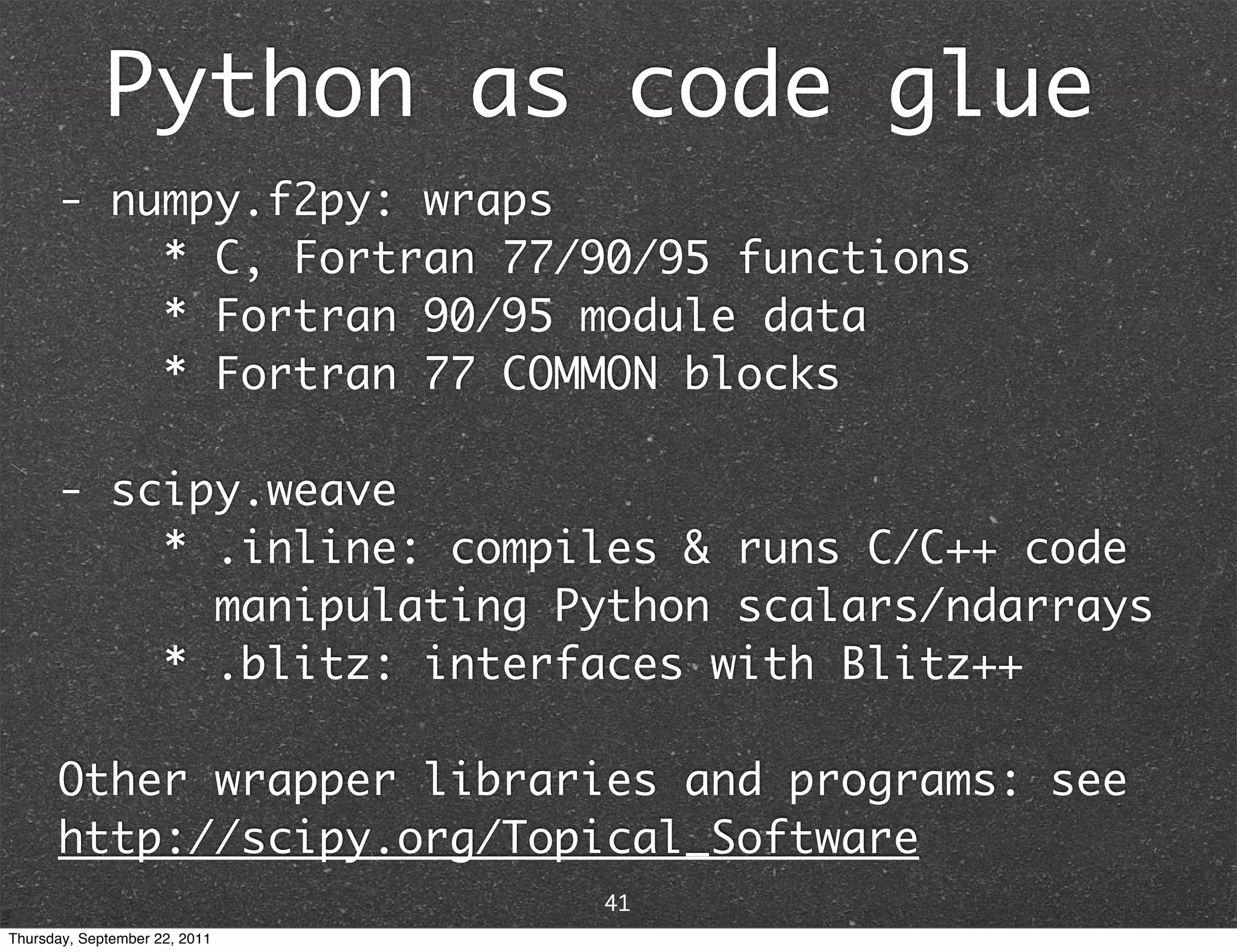
Python as code glue - numpy.f2py: wraps * C, Fortran 77/90/95 functions * Fortran 90/95 module data * Fortran 77 COMMON blocks - scipy.weave * .inline: compiles & runs C/C++ code manipulating Python scalars/ndarrays * .blitz: interfaces with Blitz++ Other wrapper libraries and programs: see http://scipy.org/Topical_Software 41 Thursday, September 22, 2011

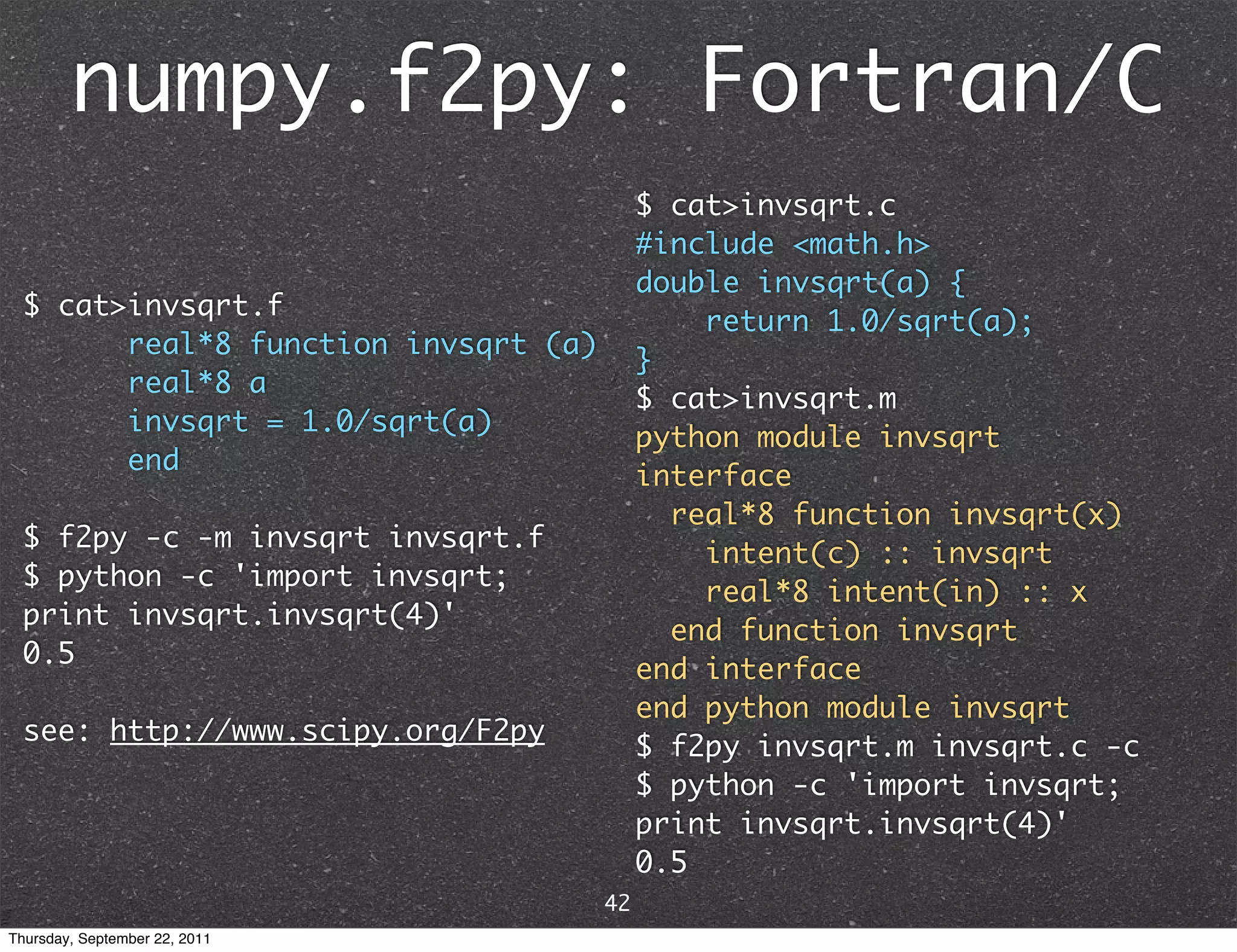
numpy.f2py: Fortran/C $ cat>invsqrt.c #include <math.h> double invsqrt(a) { $ cat>invsqrt.f return 1.0/sqrt(a); real*8 function invsqrt (a) } real*8 a $ cat>invsqrt.m invsqrt = 1.0/sqrt(a) python module invsqrt end interface real*8 function invsqrt(x) $ f2py -c -m invsqrt invsqrt.f intent(c) :: invsqrt $ python -c 'import invsqrt; real*8 intent(in) :: x print invsqrt.invsqrt(4)' end function invsqrt 0.5 end interface end python module invsqrt see: http://www.scipy.org/F2py $ f2py invsqrt.m invsqrt.c -c $ python -c 'import invsqrt; print invsqrt.invsqrt(4)' 0.5 42 Thursday, September 22, 2011

scipy.weave.inline python on-the-fly scipy distutils compiled weave core C/C++ program inline Extension >>> from scipy.weave import inline >>> x = 4.0 >>> inline('return_val = 1./sqrt(x));', ['x']) 0.5 see: https://github.com/scipy/scipy/blob/ master/scipy/weave/doc/tutorial.txt 43 Thursday, September 22, 2011

scipy.weave.blitz Uses the Blitz++ numerical library for C++ Converts between ndarrays and Blitz arrays >>> # Computes five-point average using numpy and weave.blitz >>> import numpy import empty >>> from scipy.weave import blitz >>> a = numpy.zeros((4096,4096)); c = numpy.zeros((4096, 4096)) >>> b = numpy.random.randn(4096,4096) >>> c[1:-1,1:-1] = (b[1:-1,1:-1] + b[2:,1:-1] + b[:-2,1:-1] + b [1:-1,2:] + b[1:-1,:-2]) / 5.0 >>> blitz("a[1:-1,1:-1] = (b[1:-1,1:-1] + b[2:,1:-1] + b [:-2,1:-1] + b[1:-1,2:] + b[1:-1,:-2]) / 5.") >>> (a == c).all() True see: https://github.com/scipy/scipy/blob/master/scipy/weave/doc/ tutorial.txt 44 Thursday, September 22, 2011

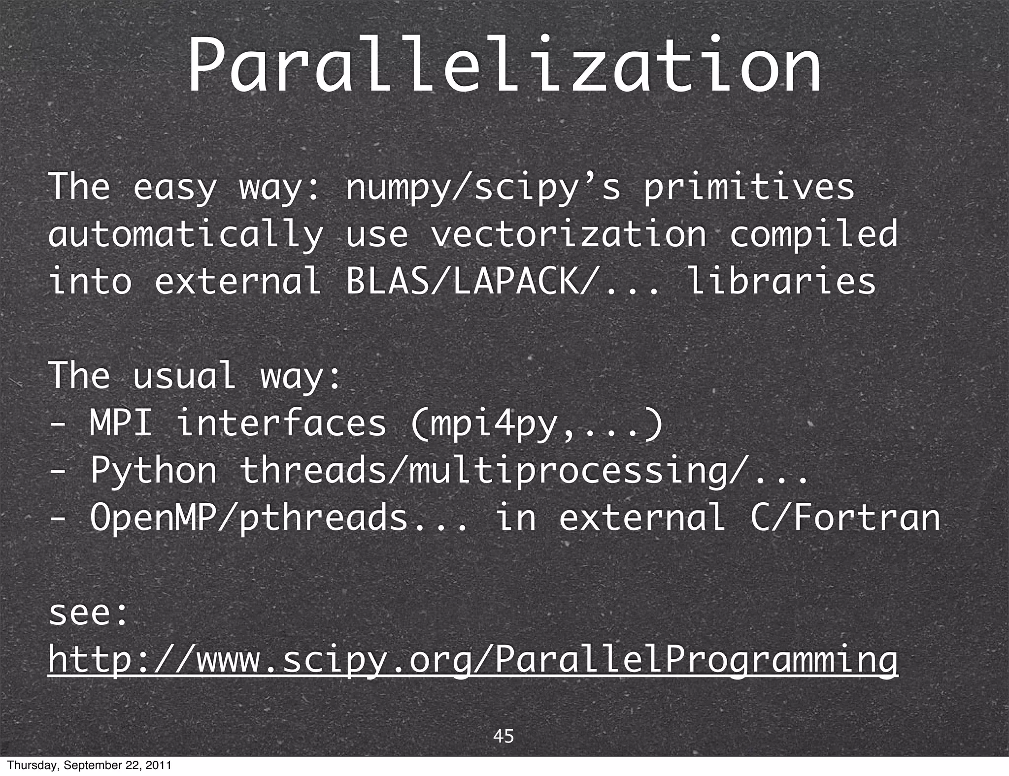
Parallelization The easy way: numpy/scipy’s primitives automatically use vectorization compiled into external BLAS/LAPACK/... libraries The usual way: - MPI interfaces (mpi4py,...) - Python threads/multiprocessing/... - OpenMP/pthreads... in external C/Fortran see: http://www.scipy.org/ParallelProgramming 45 Thursday, September 22, 2011

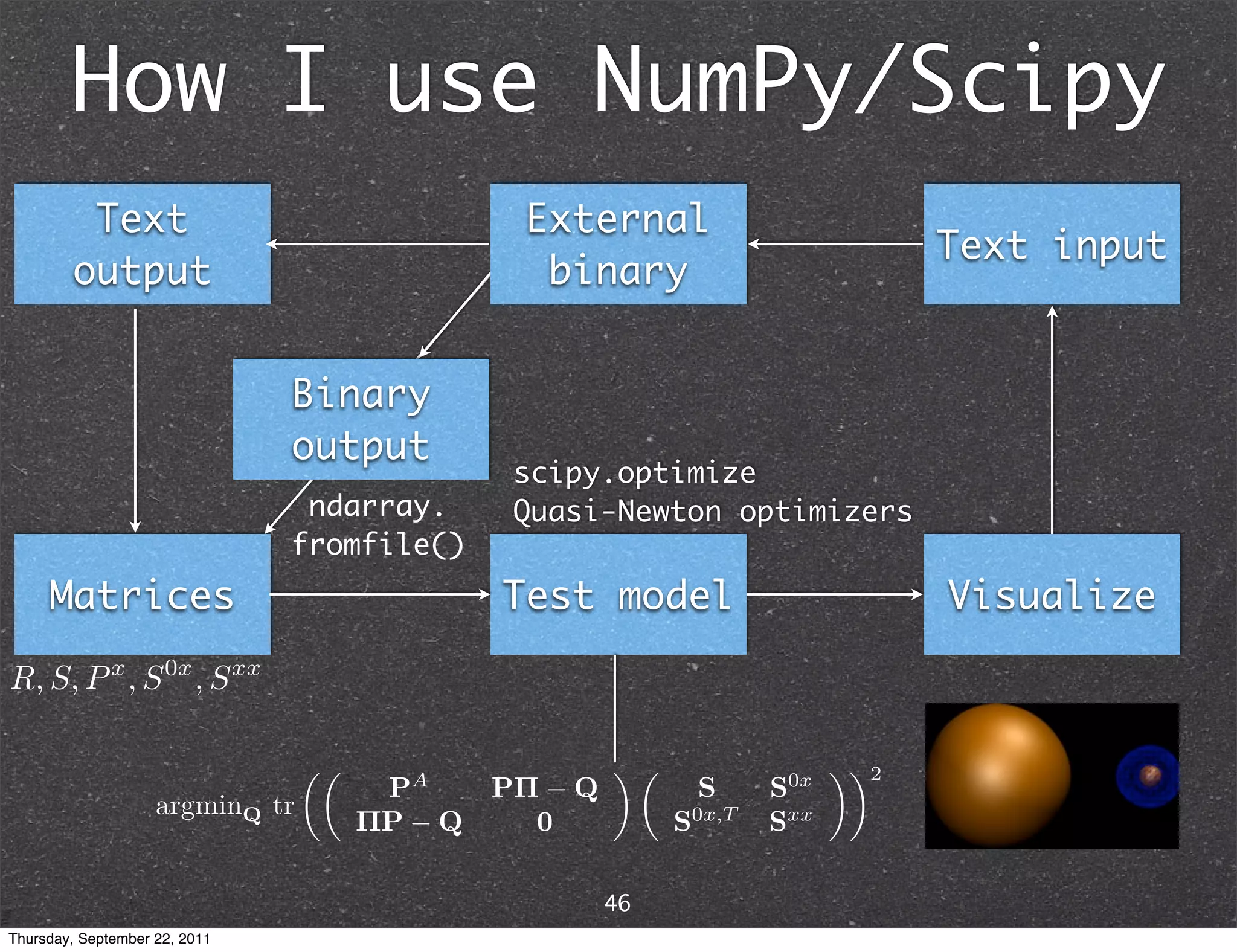
How I use NumPy/Scipy Text External Text input output binary Binary output scipy.optimize ndarray. Quasi-Newton optimizers fromfile() Matrices Test model Visualize 46 Thursday, September 22, 2011

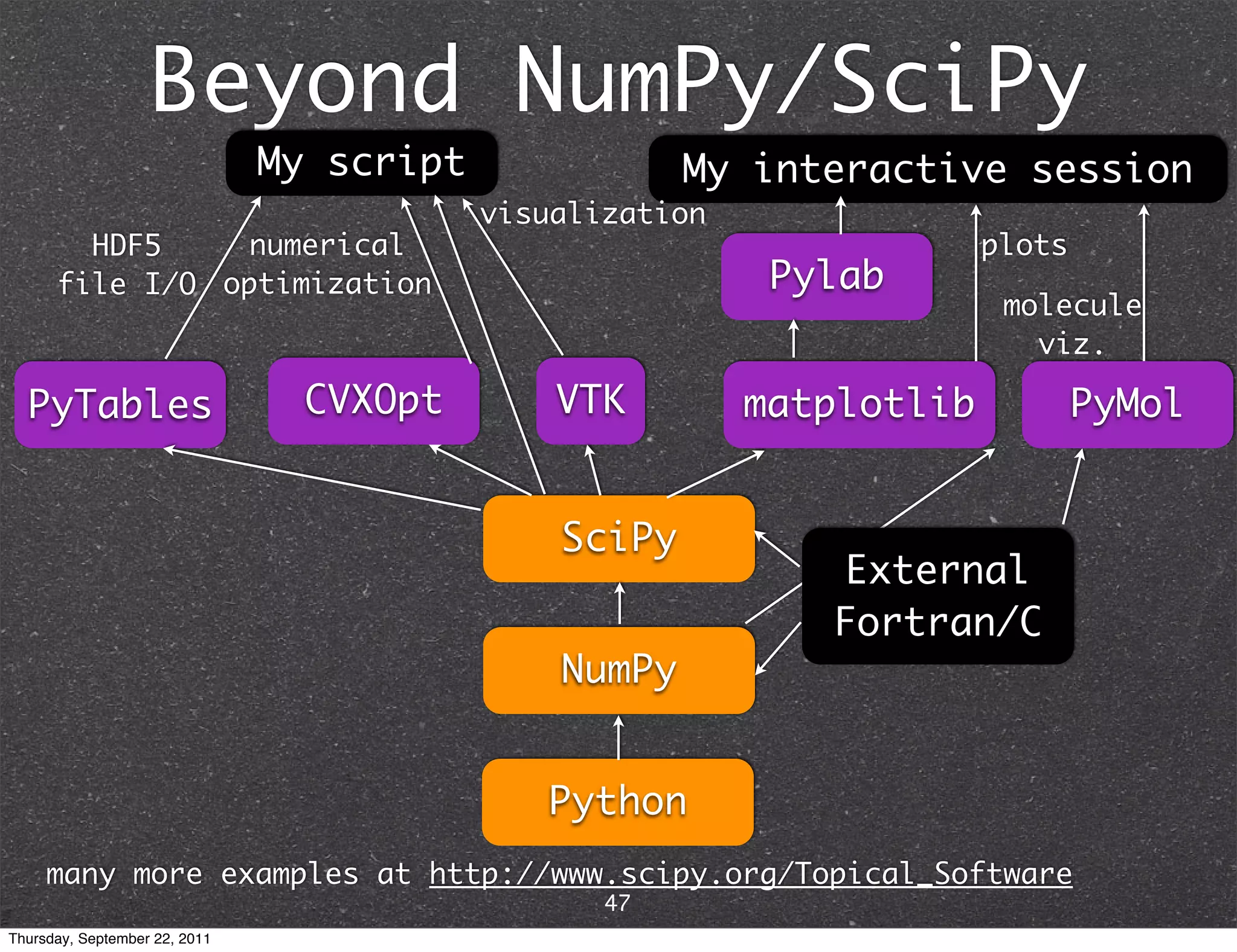
Beyond NumPy/SciPy My script My interactive session visualization HDF5 numerical plots file I/O optimization Pylab molecule viz. PyTables CVXOpt VTK matplotlib PyMol SciPy External Fortran/C NumPy Python many more examples at http://www.scipy.org/Topical_Software 47 Thursday, September 22, 2011

Python as number crunching code glue

More Related Content

What's hot

Viewers also liked

Similar to Python as number crunching code glue

Recently uploaded

Python as number crunching code glue