Naïve Bayes Classifier KeChen http://intranet.cs.man.ac.uk/mlo/comp20411/ Modified and extended by Longin Jan Latecki latecki@temple.edu
2.
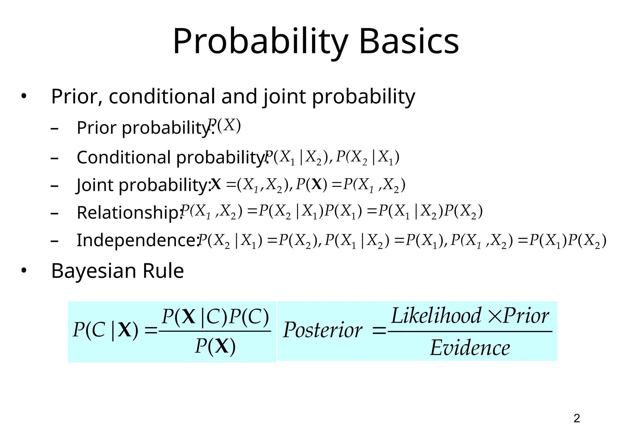
2 Probability Basics • Prior,conditional and joint probability – Prior probability: – Conditional probability: – Joint probability: – Relationship: – Independence: • Bayesian Rule ) | , ) ( 1 2 1 X P(X X | X P 2 ) ( ) ( ) ( ) ( X X X P C P C | P | C P ) (X P ) ) ( ), , ( 2 2 ,X P(X P X X 1 1 X X ) ( ) | ( ) ( ) | ( ) 2 2 1 1 1 2 2 X P X X P X P X X P ,X P(X1 ) ( ) ( ) ), ( ) | ( ), ( ) | ( 2 1 2 1 2 1 2 1 2 X P X P ,X P(X X P X X P X P X X P 1 Evidence Prior Likelihood Posterior
3.
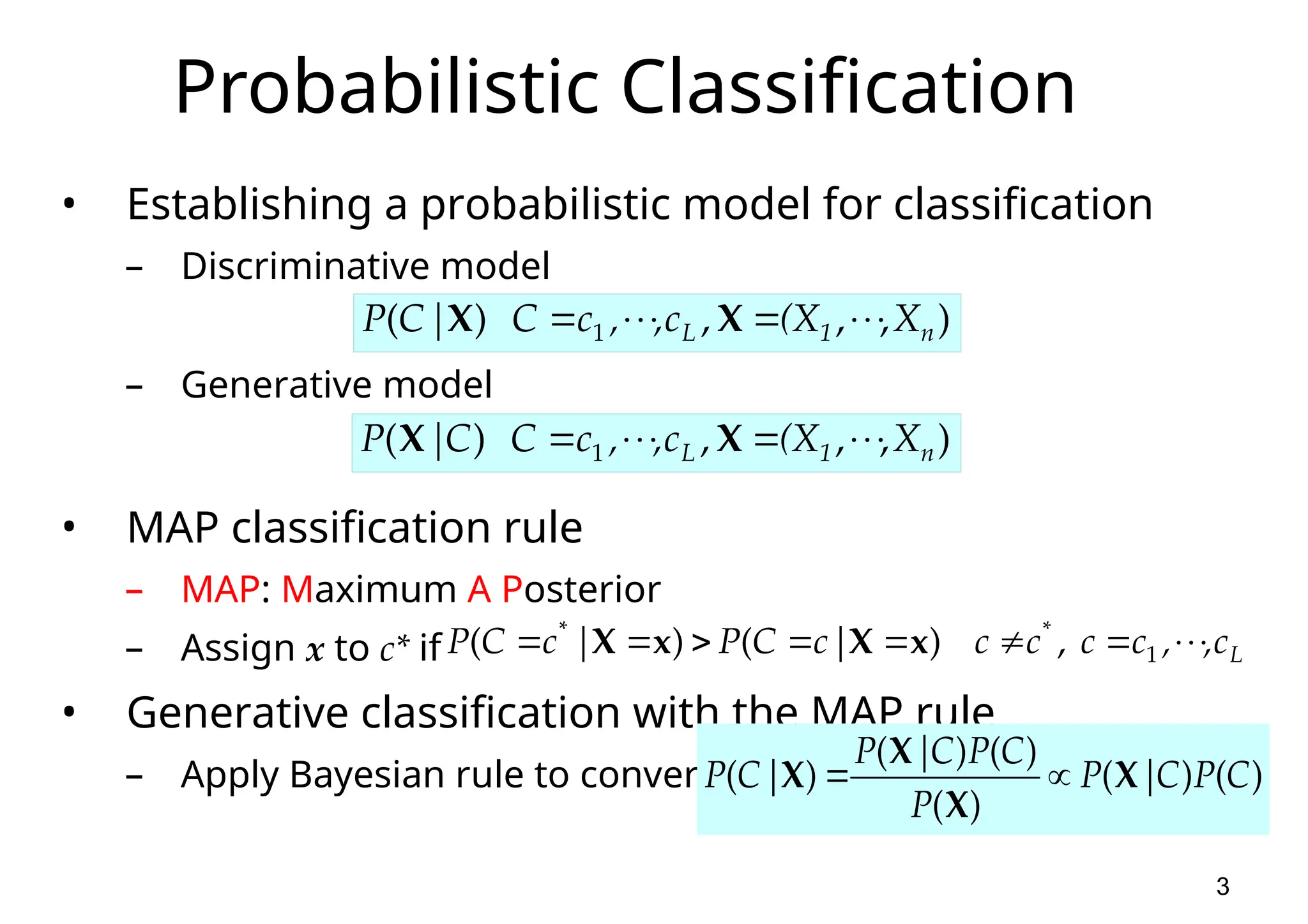
3 Probabilistic Classification • Establishinga probabilistic model for classification – Discriminative model – Generative model • MAP classification rule – MAP: Maximum A Posterior – Assign x to c* if • Generative classification with the MAP rule – Apply Bayesian rule to convert: ) , , , ) ( 1 n 1 L X (X c , , c C | C P X X ) , , , ) ( 1 n 1 L X (X c , , c C C | P X X L c , , c c c c | c C P | c C P 1 * * , ) ( ) ( x X x X ) ( ) ( ) ( ) ( ) ( ) ( C P C | P P C P C | P | C P X X X X
4.
4 Naïve Bayes • Bayesclassification Difficulty: learning the joint probability • Naïve Bayes classification – Making the assumption that all input attributes are independent – MAP classification rule ) ( ) | , , ( ) ( ) ( ) ( 1 C P C X X P C P C | P | C P n X X ) | , , ( 1 C X X P n ) | ( ) | ( ) | ( ) | , , ( ) | ( ) | , , ( ) ; , , | ( ) | , , , ( 2 1 2 1 2 2 1 2 1 C X P C X P C X P C X X P C X P C X X P C X X X P C X X X P n n n n n L n n c c c c c c P c x P c x P c P c x P c x P , , , ), ( )] | ( ) | ( [ ) ( )] | ( ) | ( [ 1 * 1 * * * 1 L c , , c c c c | c C P | c C P 1 * * , ) ( ) ( x X x X
5.
5 Naïve Bayes • NaïveBayes Algorithm (for discrete input attributes) – Learning Phase: Given a training set S, Output: conditional probability tables; for elements – Test Phase: Given an unknown instance , Look up tables to assign the label c* to X’ if ; in examples with ) | ( estimate ) | ( ˆ ) , 1 ; , , 1 ( attribute each of value attribute every For ; in examples with ) ( estimate ) ( ˆ of value target each For 1 S S i jk j i jk j j j jk i i L i i c C a X P c C a X P N , k n j x a c C P c C P ) c , , c (c c L n n c c c c c c P c a P c a P c P c a P c a P , , , ), ( ˆ )] | ( ˆ ) | ( ˆ [ ) ( ˆ )] | ( ˆ ) | ( ˆ [ 1 * 1 * * * 1 ) , , ( 1 n a a X L N x j j ,
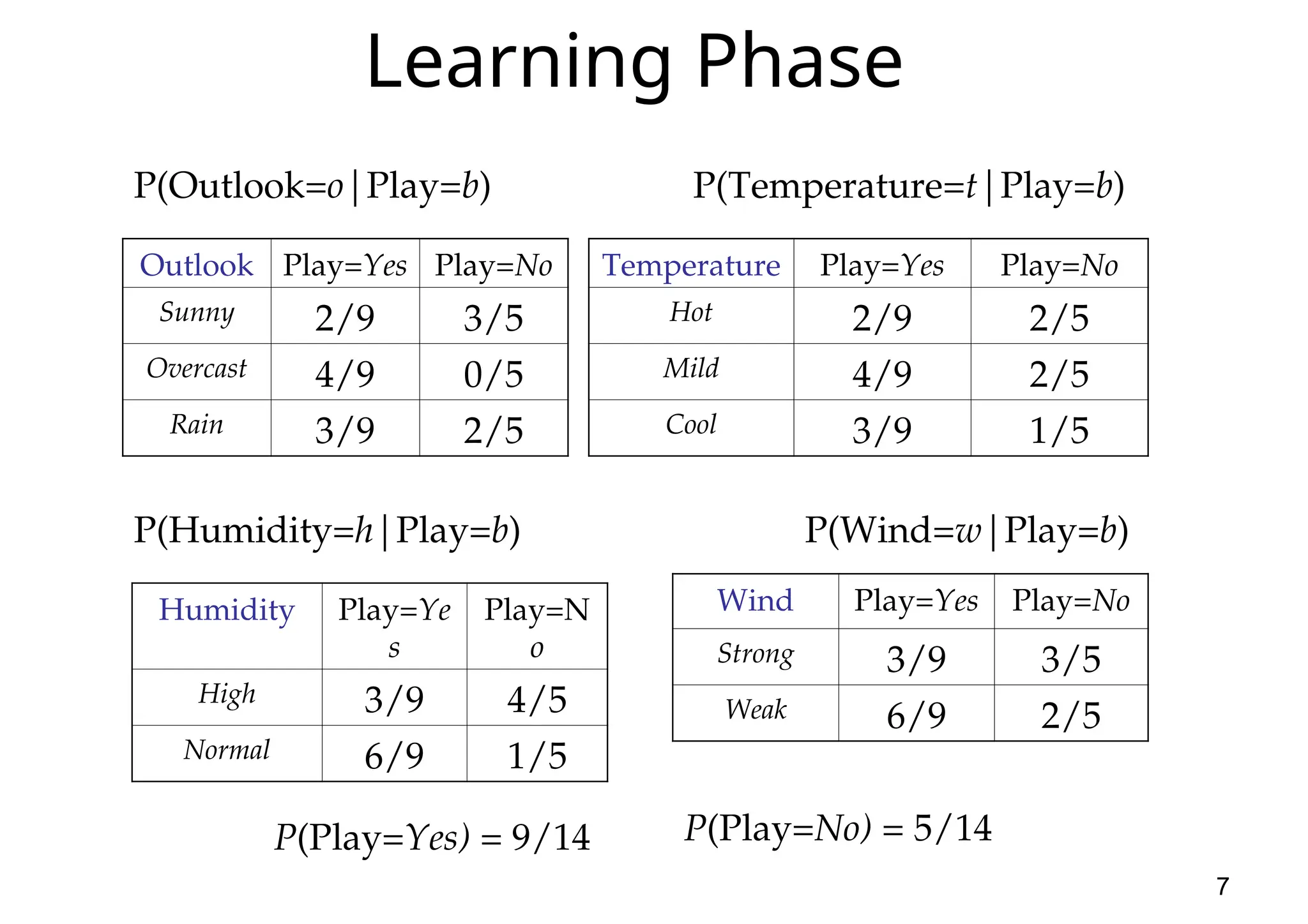
7 Learning Phase Outlook Play=YesPlay=No Sunny 2/9 3/5 Overcast 4/9 0/5 Rain 3/9 2/5 Temperature Play=Yes Play=No Hot 2/9 2/5 Mild 4/9 2/5 Cool 3/9 1/5 Humidity Play=Ye s Play=N o High 3/9 4/5 Normal 6/9 1/5 Wind Play=Yes Play=No Strong 3/9 3/5 Weak 6/9 2/5 P(Play=Yes) = 9/14 P(Play=No) = 5/14 P(Outlook=o|Play=b) P(Temperature=t|Play=b) P(Humidity=h|Play=b) P(Wind=w|Play=b)
8.
8 Example • Test Phase –Given a new instance x’, P(Play =Yes|x’) ? P(Play = No|x’) x’=(Outlook=Sunny, Temperature=Cool, Humidity=High, Wind=Strong) – Look up tables – MAP rule P(Outlook=Sunny|Play=No) = 3/5 P(Temperature=Cool|Play==No) = 1/5 P(Huminity=High|Play=No) = 4/5 P(Wind=Strong|Play=No) = 3/5 P(Play=No) = 5/14 P(Outlook=Sunny|Play=Yes) = 2/9 P(Temperature=Cool|Play=Yes) = 3/9 P(Huminity=High|Play=Yes) = 3/9 P(Wind=Strong|Play=Yes) = 3/9 P(Play=Yes) = 9/14 P(Play=Yes|x’): [P(Sunny|Yes)P(Cool|Yes)P(High|Yes)P(Strong|Yes)]P(Play=Yes) = 0.0053 P(Play=No|x’): [P(Sunny|No) P(Cool|No)P(High|No)P(Strong|No)]P(Play=No) = 0.0206 Given the fact P(Play =Yes|x’) < P(Play = No|x’), we label x’ to be “No”.
9.
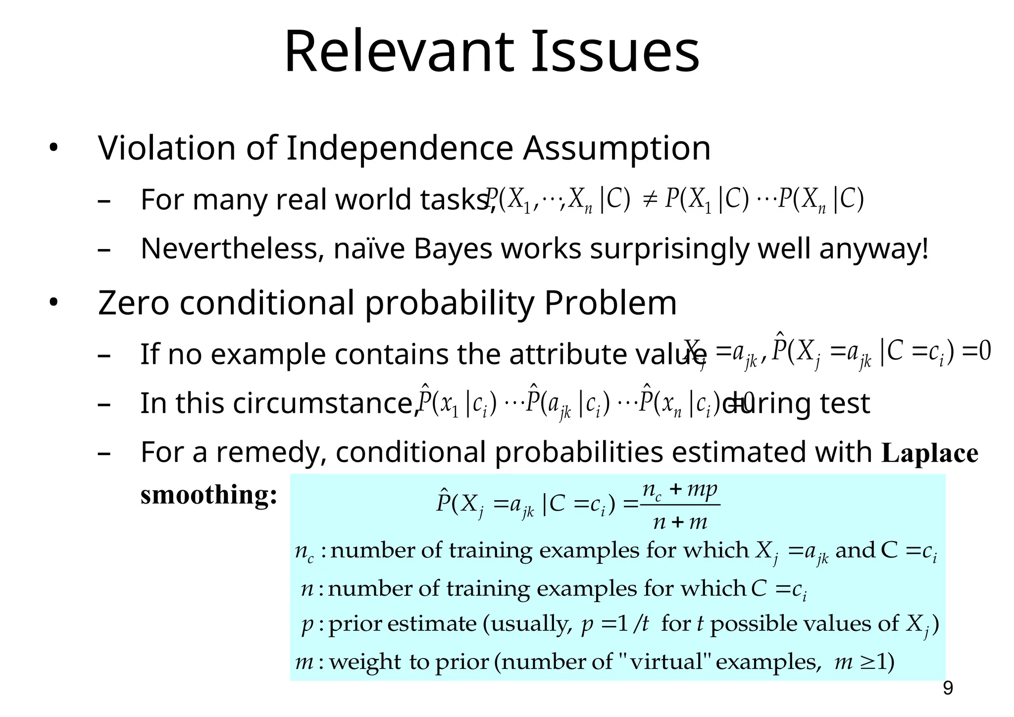
9 Relevant Issues • Violationof Independence Assumption – For many real world tasks, – Nevertheless, naïve Bayes works surprisingly well anyway! • Zero conditional probability Problem – If no example contains the attribute value – In this circumstance, during test – For a remedy, conditional probabilities estimated with Laplace smoothing: ) | ( ) | ( ) | , , ( 1 1 C X P C X P C X X P n n 0 ) | ( ˆ , i jk j jk j c C a X P a X 0 ) | ( ˆ ) | ( ˆ ) | ( ˆ 1 i n i jk i c x P c a P c x P ) 1 examples, virtual" " of (number prior to weight : ) of values possible for / 1 (usually, estimate prior : which for examples training of number : C and which for examples training of number : ) | ( ˆ m m X t t p p c C n c a X n m n mp n c C a X P j i i jk j c c i jk j
10.
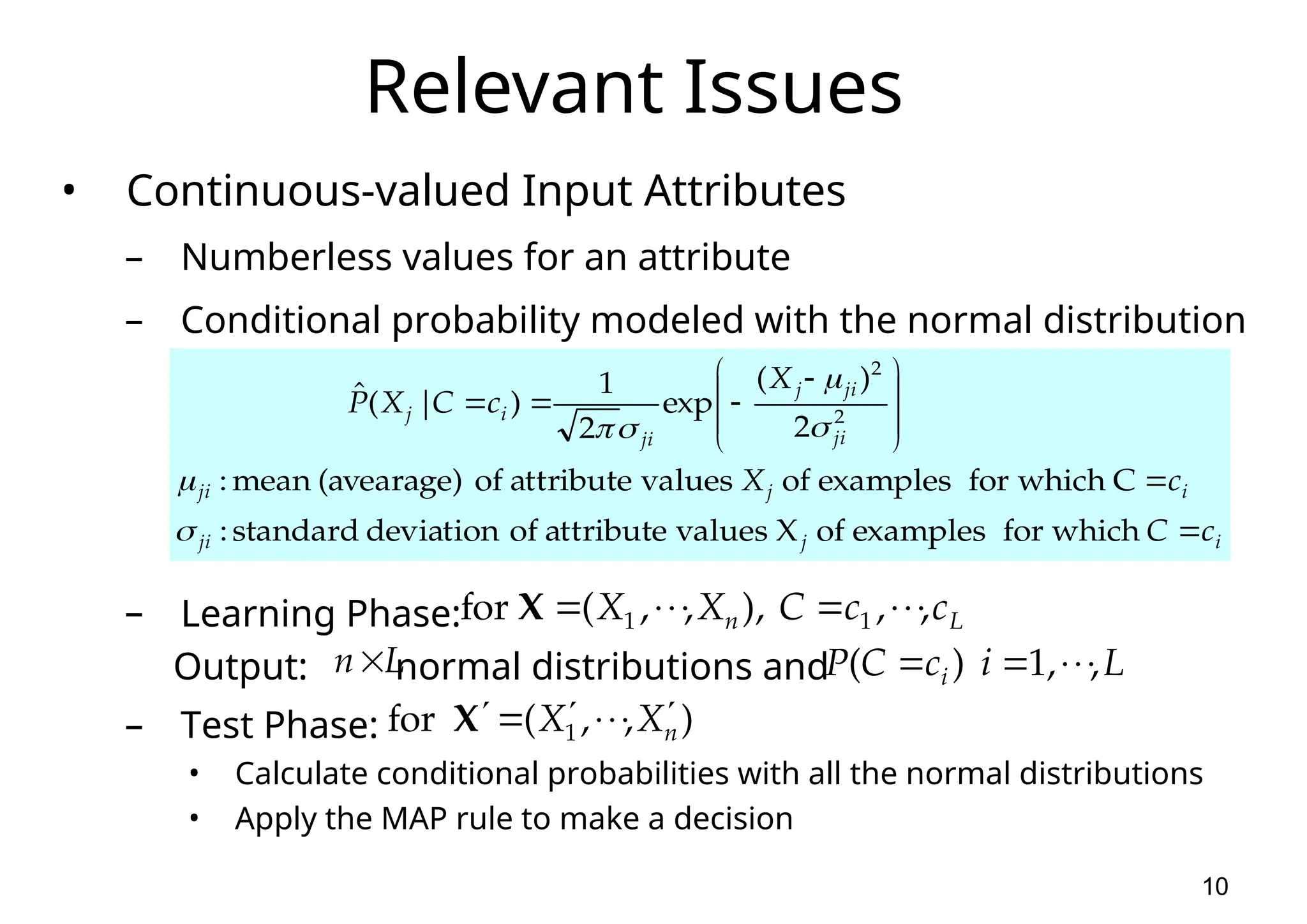
10 Relevant Issues • Continuous-valuedInput Attributes – Numberless values for an attribute – Conditional probability modeled with the normal distribution – Learning Phase: Output: normal distributions and – Test Phase: • Calculate conditional probabilities with all the normal distributions • Apply the MAP rule to make a decision i j ji i j ji ji ji j ji i j c C c X X c C X P which for examples of X values attribute of deviation standard : C which for examples of values attribute of (avearage) mean : 2 ) ( exp 2 1 ) | ( ˆ 2 2 L n c c C X X , , ), , , ( for 1 1 X L n ) , , ( for 1 n X X X L i c C P i , , 1 ) (
11.
11 Conclusions • Naïve Bayesbased on the independence assumption – Training is very easy and fast; just requiring considering each attribute in each class separately – Test is straightforward; just looking up tables or calculating conditional probabilities with normal distributions • A popular generative model – Performance competitive to most of state-of-the-art classifiers even in presence of violating independence assumption – Many successful applications, e.g., spam mail filtering – Apart from classification, naïve Bayes can do more…
12.
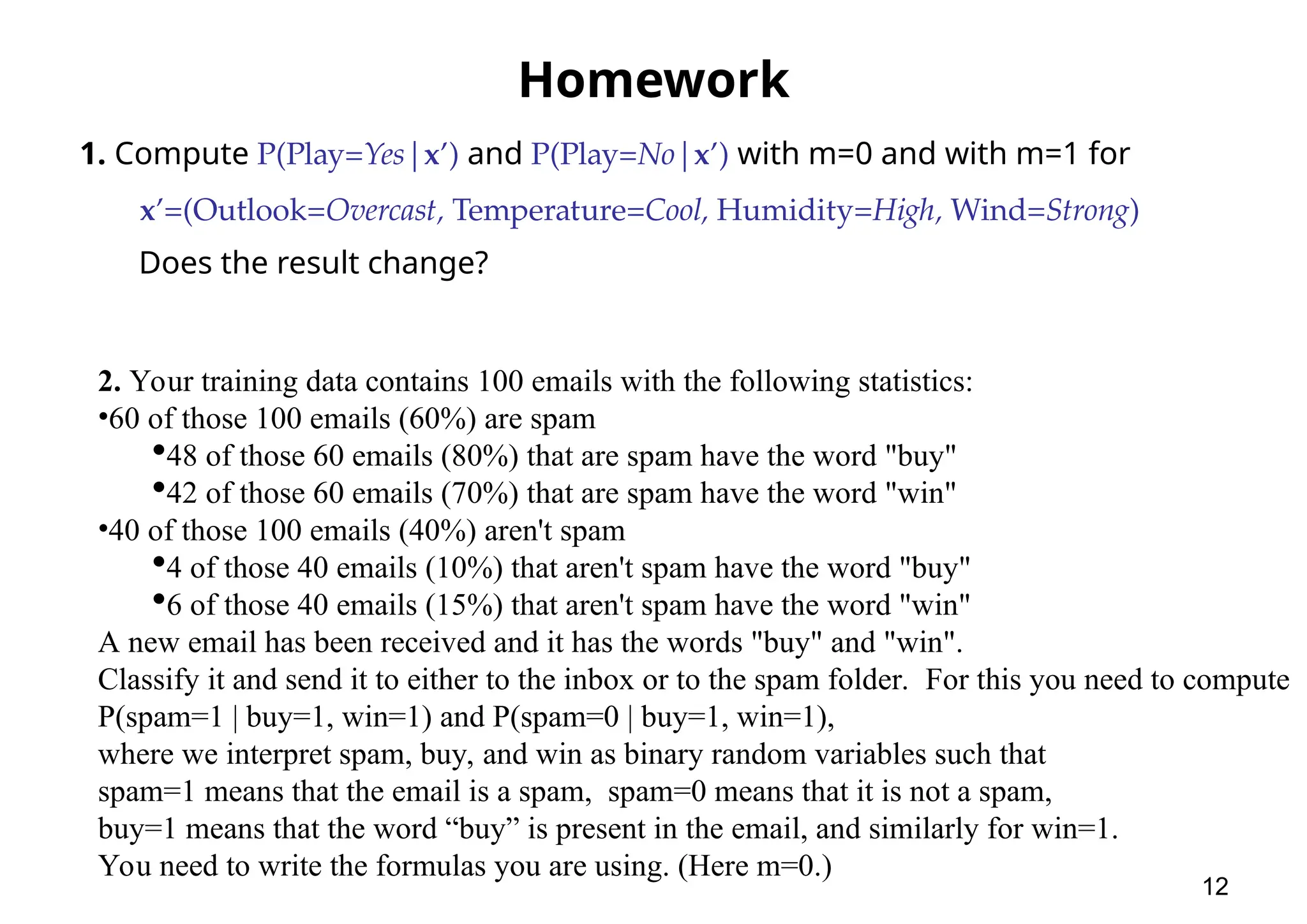
Homework 1. Compute P(Play=Yes|x’)and P(Play=No|x’) with m=0 and with m=1 for x’=(Outlook=Overcast, Temperature=Cool, Humidity=High, Wind=Strong) Does the result change? 12 2. Your training data contains 100 emails with the following statistics: •60 of those 100 emails (60%) are spam 48 of those 60 emails (80%) that are spam have the word "buy" 42 of those 60 emails (70%) that are spam have the word "win" •40 of those 100 emails (40%) aren't spam 4 of those 40 emails (10%) that aren't spam have the word "buy" 6 of those 40 emails (15%) that aren't spam have the word "win" A new email has been received and it has the words "buy" and "win". Classify it and send it to either to the inbox or to the spam folder. For this you need to compute P(spam=1 | buy=1, win=1) and P(spam=0 | buy=1, win=1), where we interpret spam, buy, and win as binary random variables such that spam=1 means that the email is a spam, spam=0 means that it is not a spam, buy=1 means that the word “buy” is present in the email, and similarly for win=1. You need to write the formulas you are using. (Here m=0.)
![4 Naïve Bayes • Bayes classification Difficulty: learning the joint probability • Naïve Bayes classification – Making the assumption that all input attributes are independent – MAP classification rule ) ( ) | , , ( ) ( ) ( ) ( 1 C P C X X P C P C | P | C P n X X ) | , , ( 1 C X X P n ) | ( ) | ( ) | ( ) | , , ( ) | ( ) | , , ( ) ; , , | ( ) | , , , ( 2 1 2 1 2 2 1 2 1 C X P C X P C X P C X X P C X P C X X P C X X X P C X X X P n n n n n L n n c c c c c c P c x P c x P c P c x P c x P , , , ), ( )] | ( ) | ( [ ) ( )] | ( ) | ( [ 1 * 1 * * * 1 L c , , c c c c | c C P | c C P 1 * * , ) ( ) ( x X x X](https://image.slidesharecdn.com/naivebayes-250601113733-eae474f3/75/NaiveBayes_machine-learning-basic_ppt-ppt-4-2048.jpg)
![5 Naïve Bayes • Naïve Bayes Algorithm (for discrete input attributes) – Learning Phase: Given a training set S, Output: conditional probability tables; for elements – Test Phase: Given an unknown instance , Look up tables to assign the label c* to X’ if ; in examples with ) | ( estimate ) | ( ˆ ) , 1 ; , , 1 ( attribute each of value attribute every For ; in examples with ) ( estimate ) ( ˆ of value target each For 1 S S i jk j i jk j j j jk i i L i i c C a X P c C a X P N , k n j x a c C P c C P ) c , , c (c c L n n c c c c c c P c a P c a P c P c a P c a P , , , ), ( ˆ )] | ( ˆ ) | ( ˆ [ ) ( ˆ )] | ( ˆ ) | ( ˆ [ 1 * 1 * * * 1 ) , , ( 1 n a a X L N x j j ,](https://image.slidesharecdn.com/naivebayes-250601113733-eae474f3/75/NaiveBayes_machine-learning-basic_ppt-ppt-5-2048.jpg)
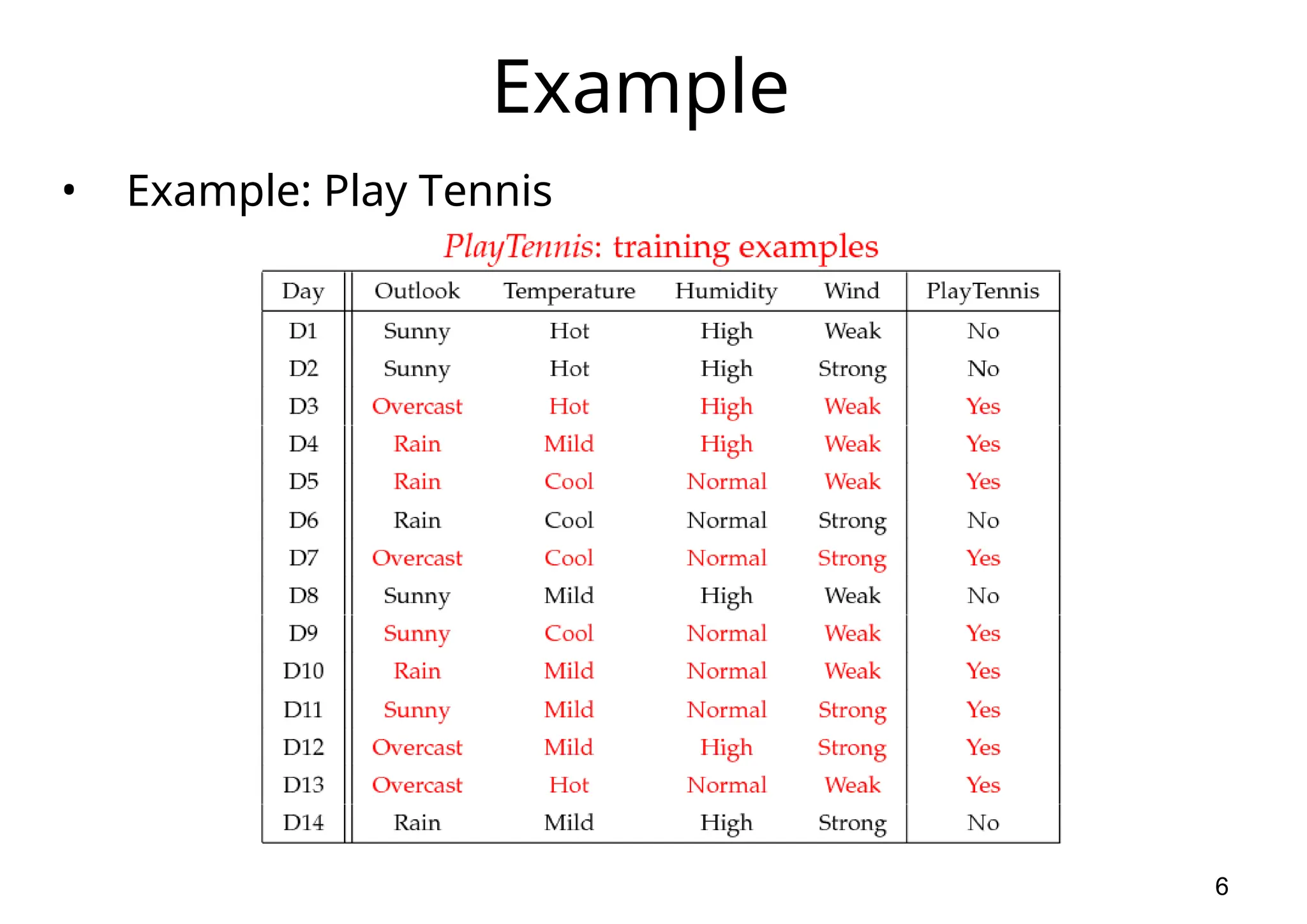
![8 Example • Test Phase – Given a new instance x’, P(Play =Yes|x’) ? P(Play = No|x’) x’=(Outlook=Sunny, Temperature=Cool, Humidity=High, Wind=Strong) – Look up tables – MAP rule P(Outlook=Sunny|Play=No) = 3/5 P(Temperature=Cool|Play==No) = 1/5 P(Huminity=High|Play=No) = 4/5 P(Wind=Strong|Play=No) = 3/5 P(Play=No) = 5/14 P(Outlook=Sunny|Play=Yes) = 2/9 P(Temperature=Cool|Play=Yes) = 3/9 P(Huminity=High|Play=Yes) = 3/9 P(Wind=Strong|Play=Yes) = 3/9 P(Play=Yes) = 9/14 P(Play=Yes|x’): [P(Sunny|Yes)P(Cool|Yes)P(High|Yes)P(Strong|Yes)]P(Play=Yes) = 0.0053 P(Play=No|x’): [P(Sunny|No) P(Cool|No)P(High|No)P(Strong|No)]P(Play=No) = 0.0206 Given the fact P(Play =Yes|x’) < P(Play = No|x’), we label x’ to be “No”.](https://image.slidesharecdn.com/naivebayes-250601113733-eae474f3/75/NaiveBayes_machine-learning-basic_ppt-ppt-8-2048.jpg)