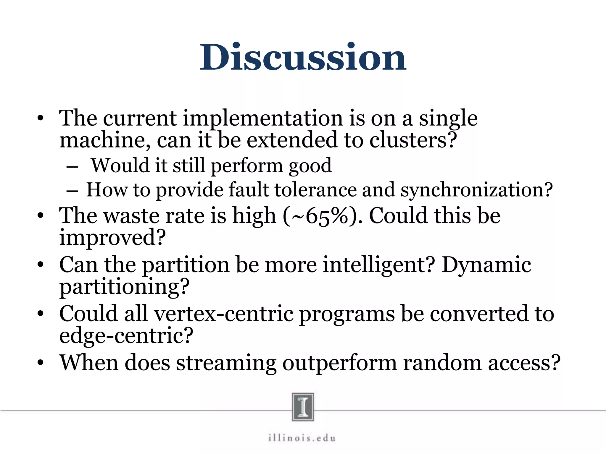
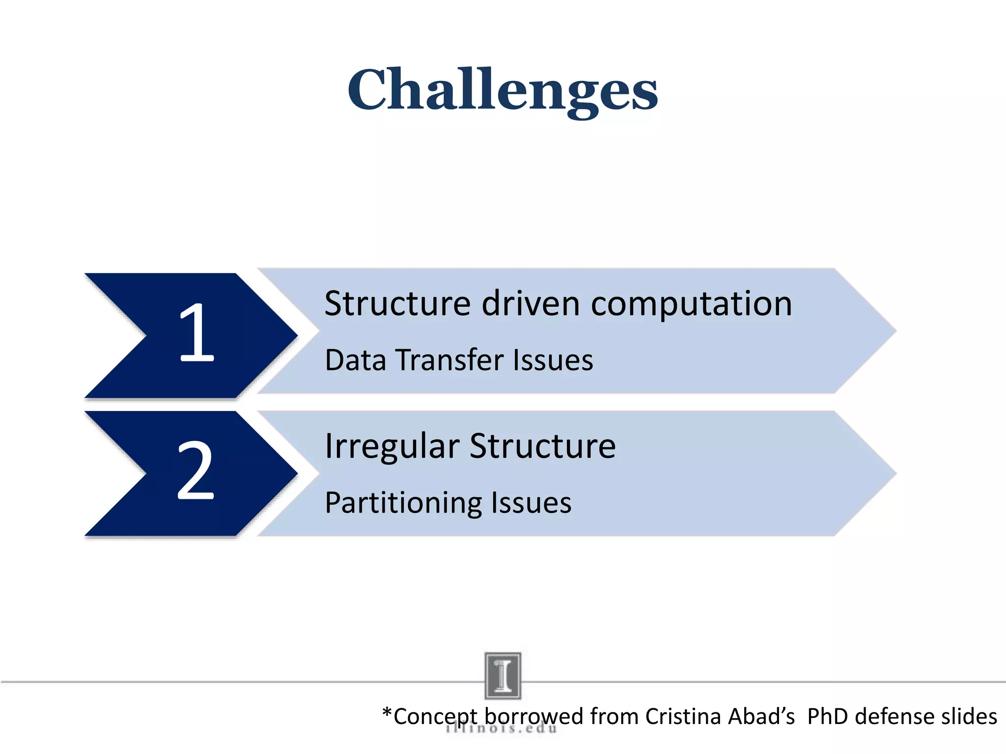
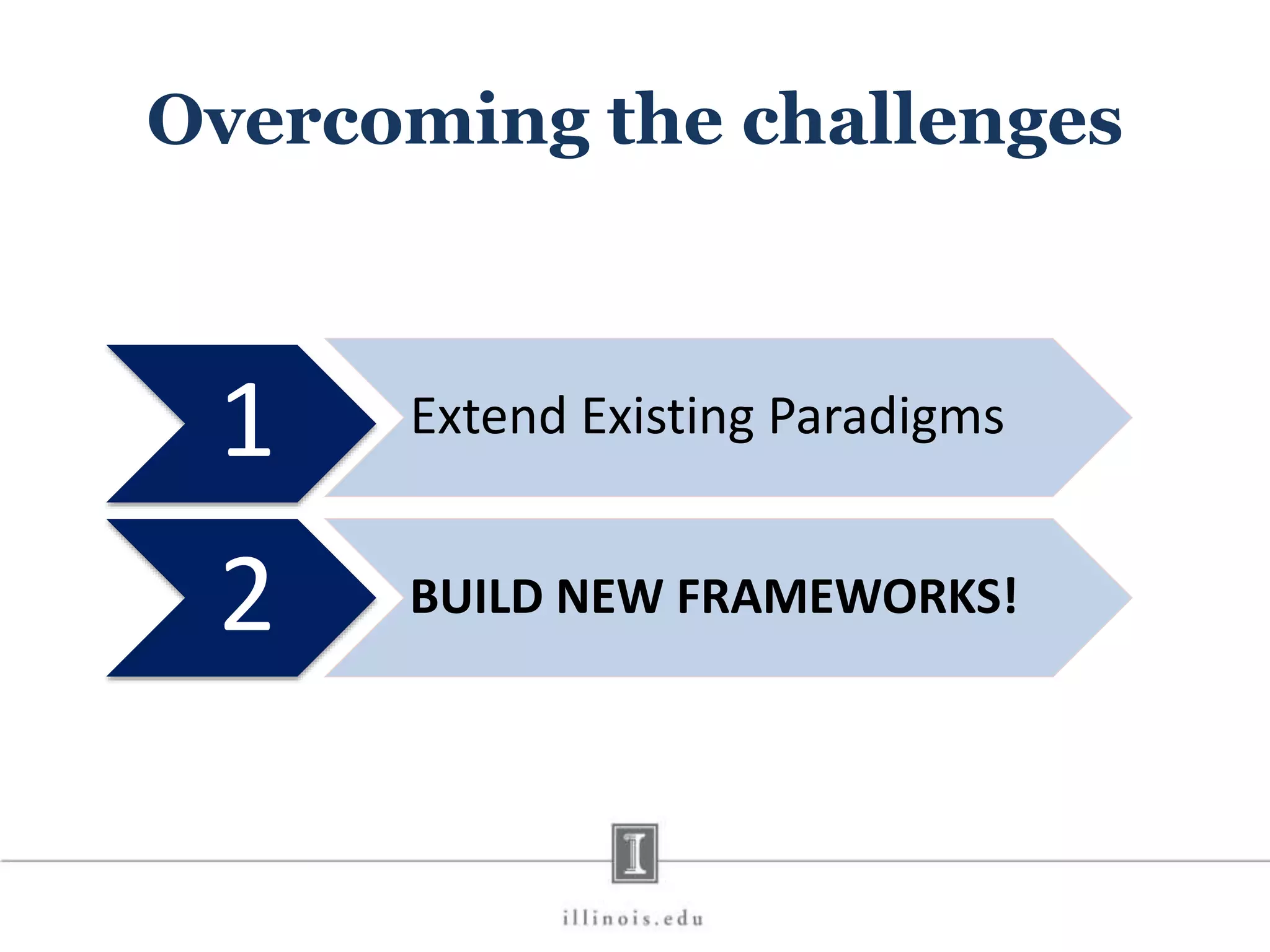
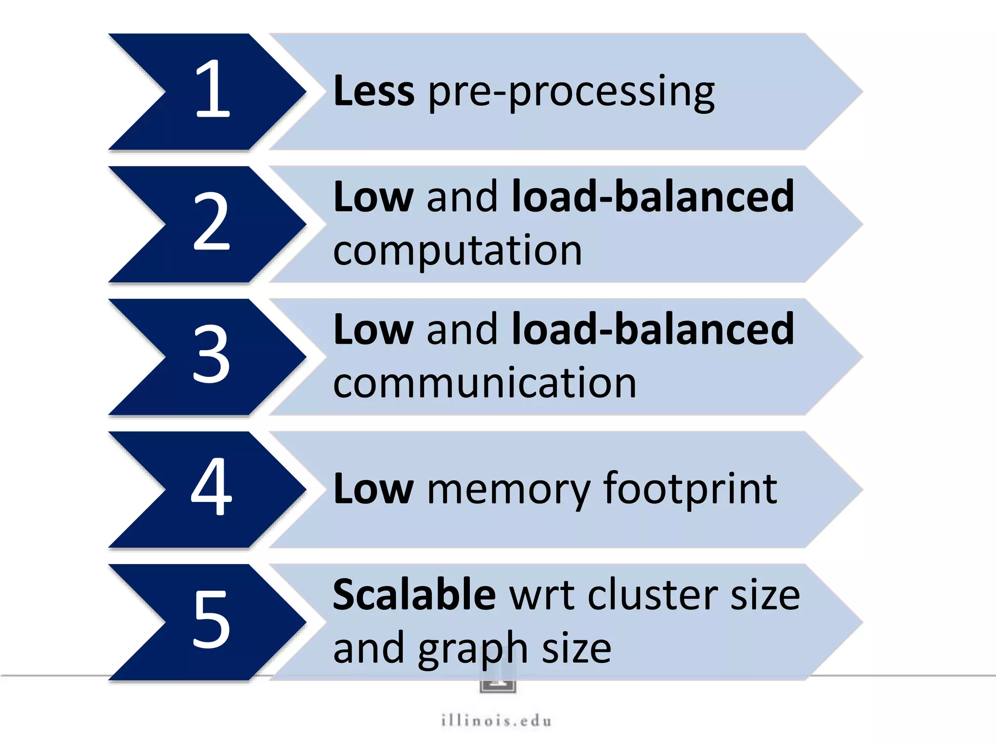
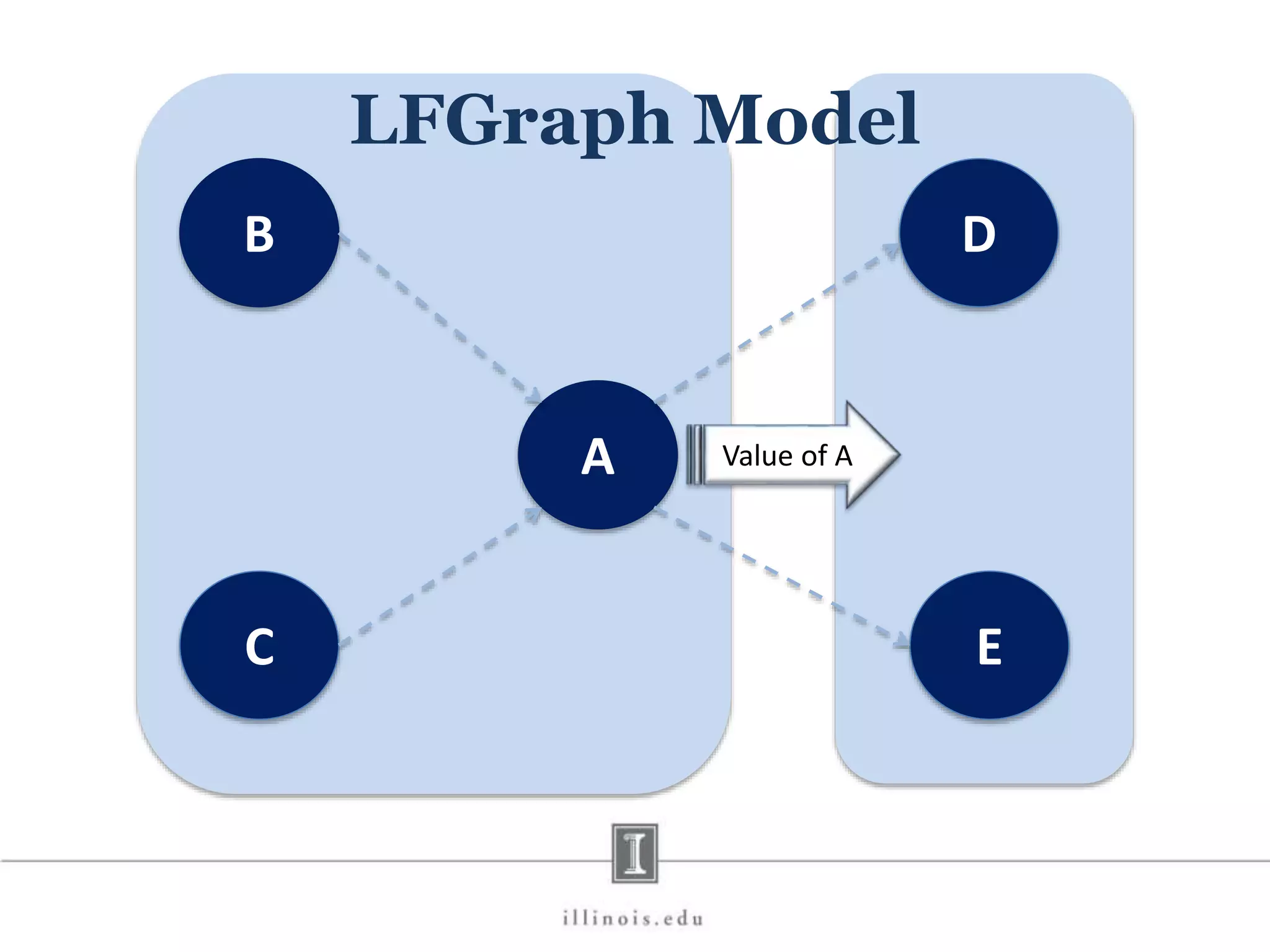
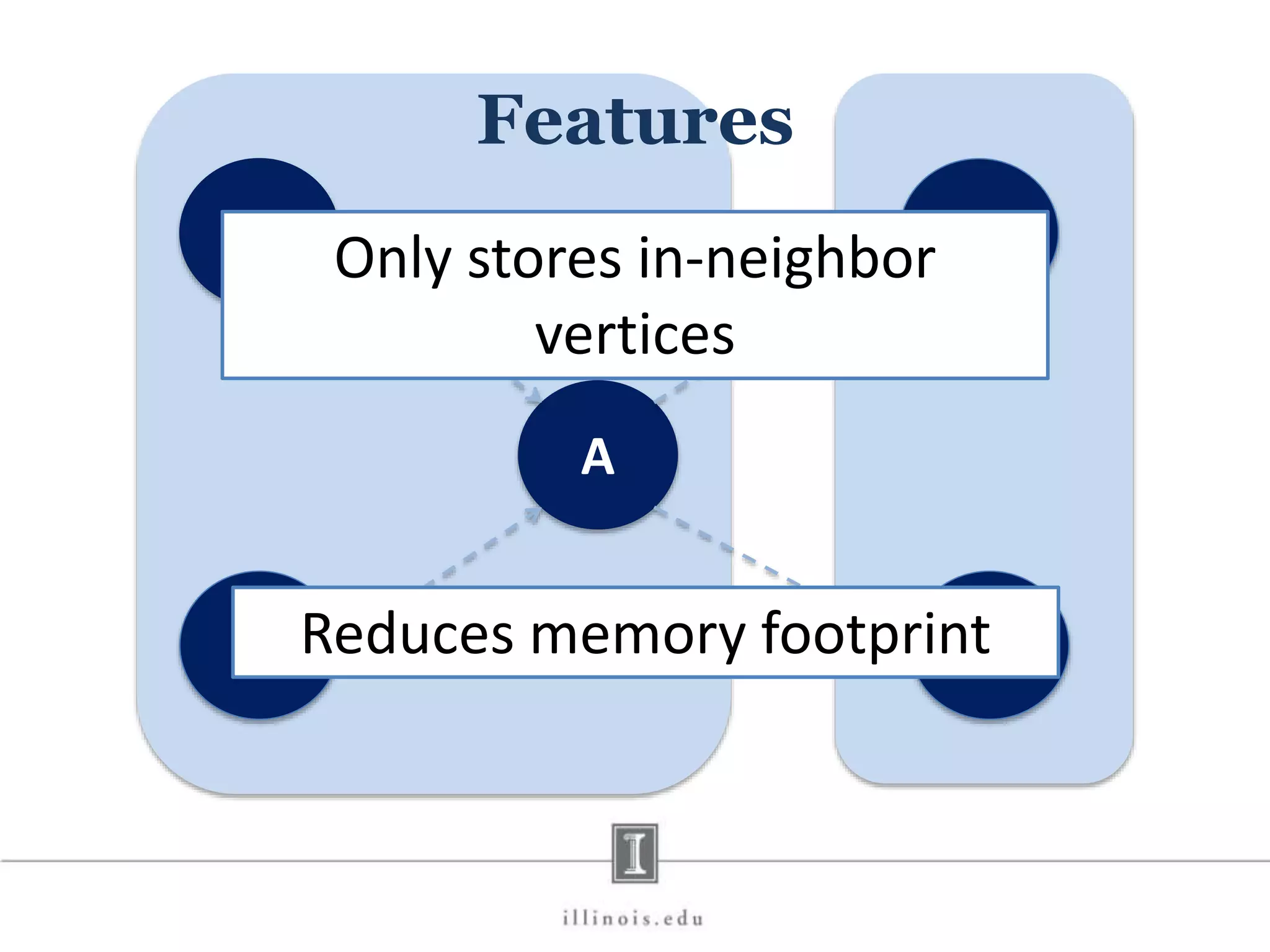
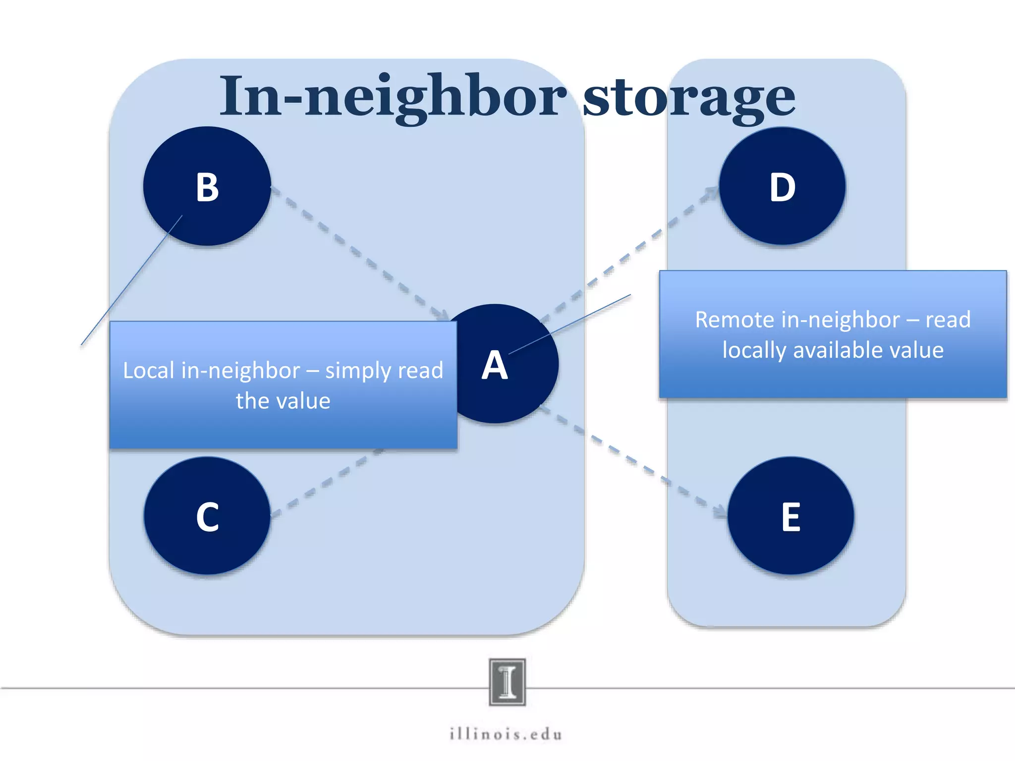
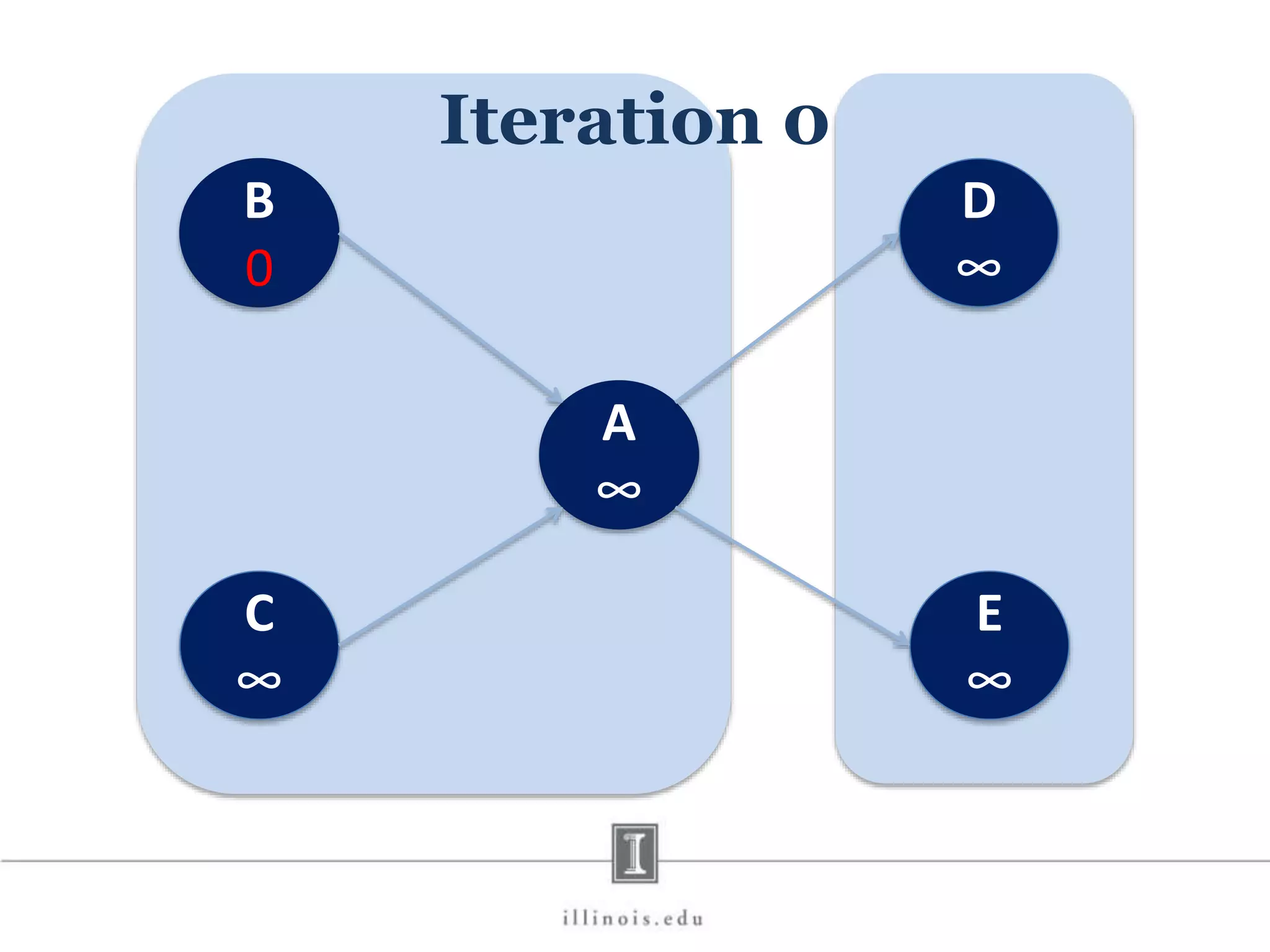
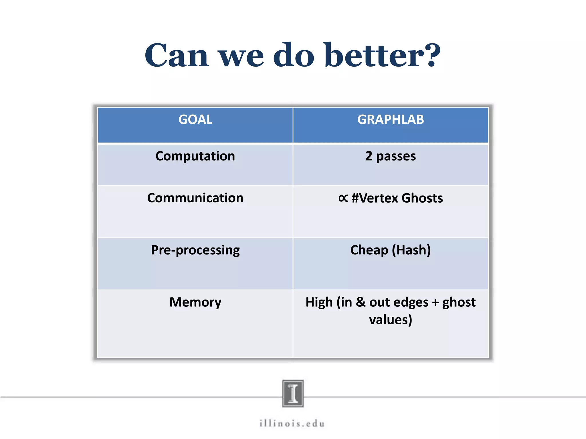
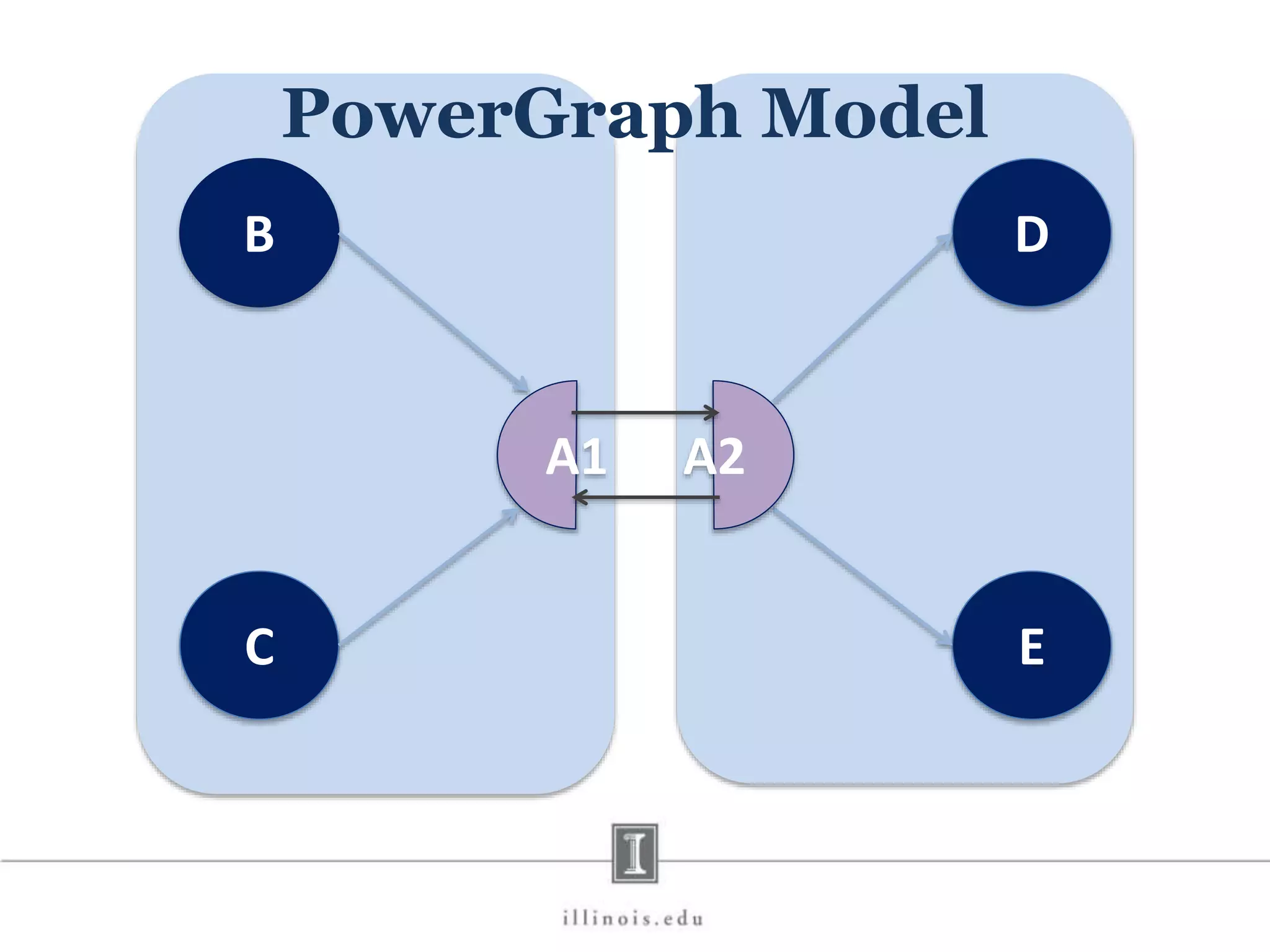
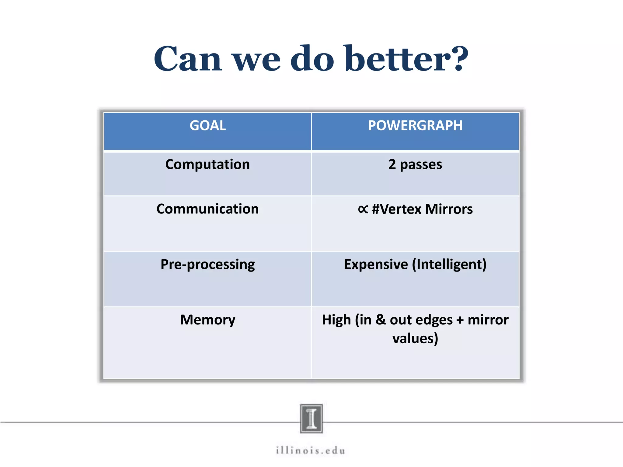
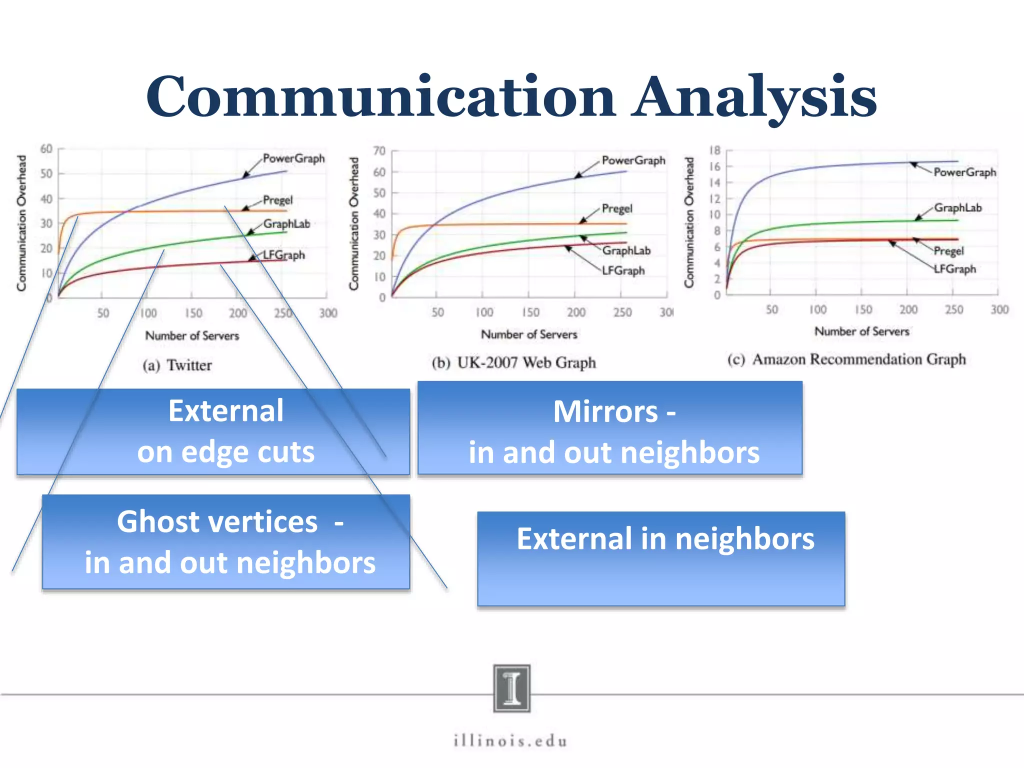
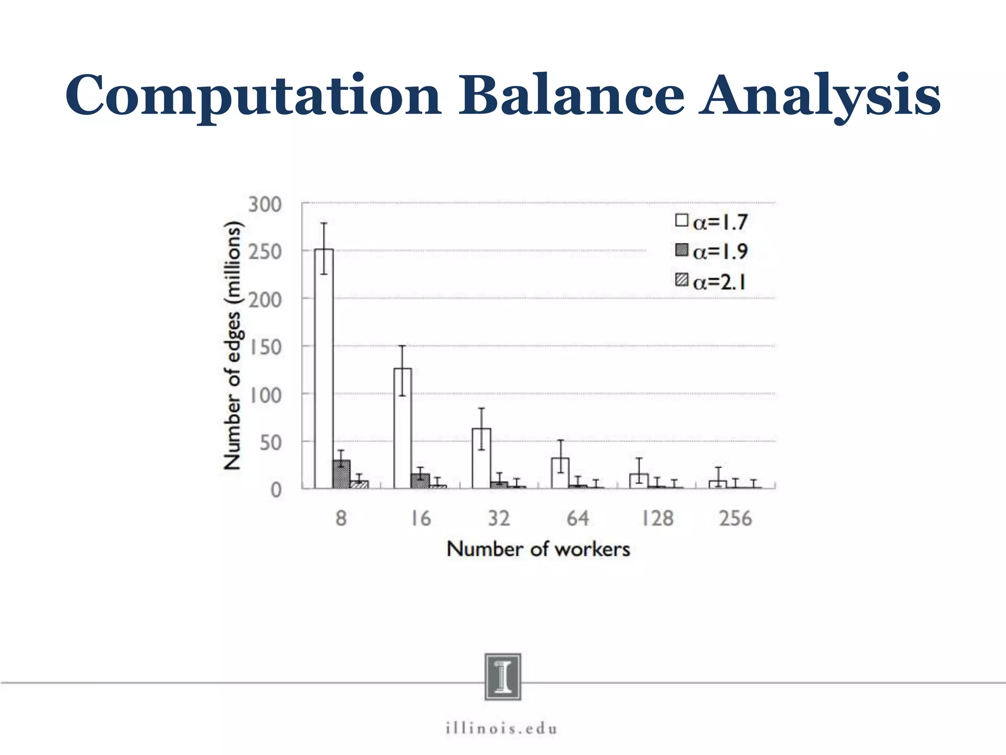
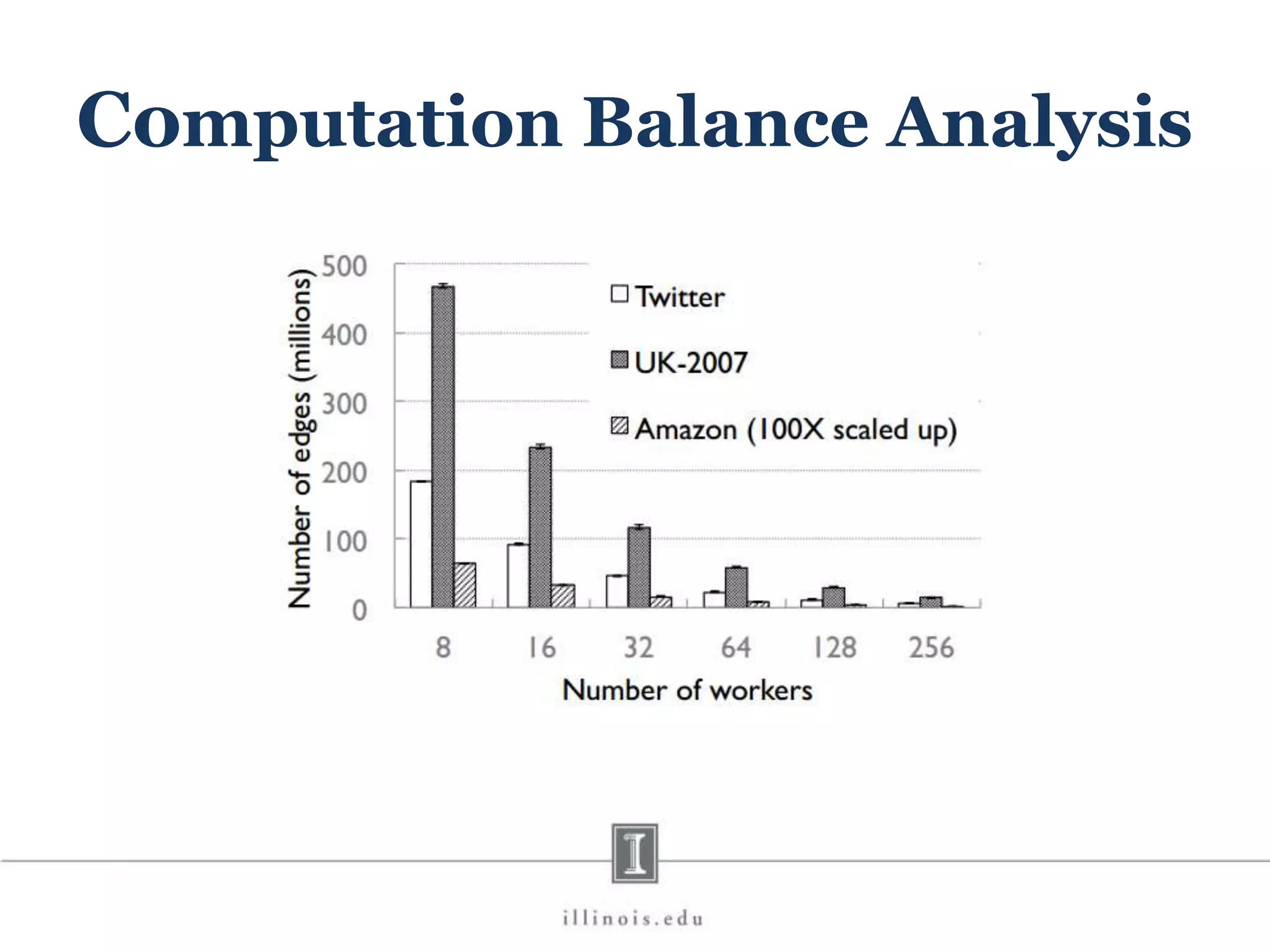
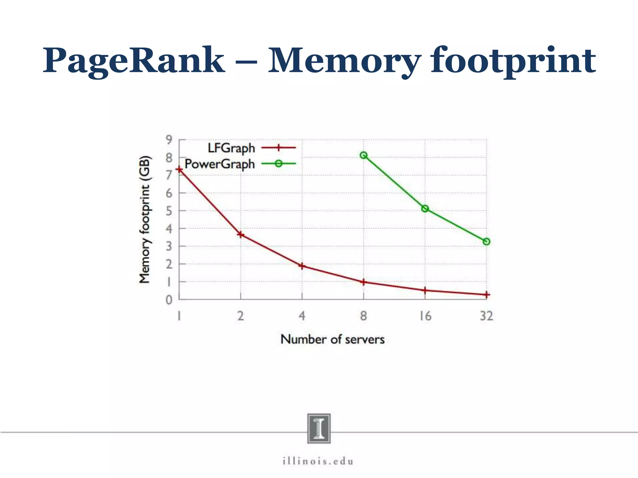
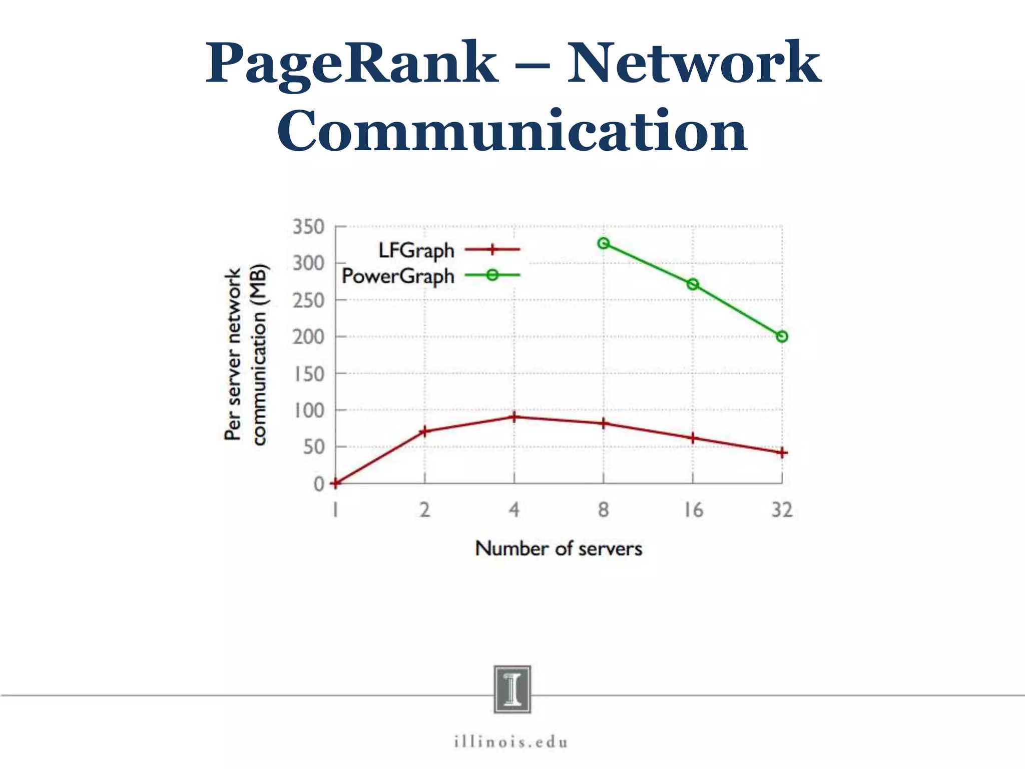
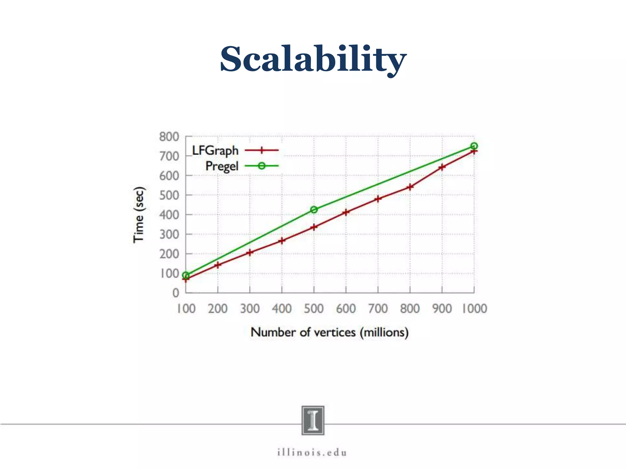
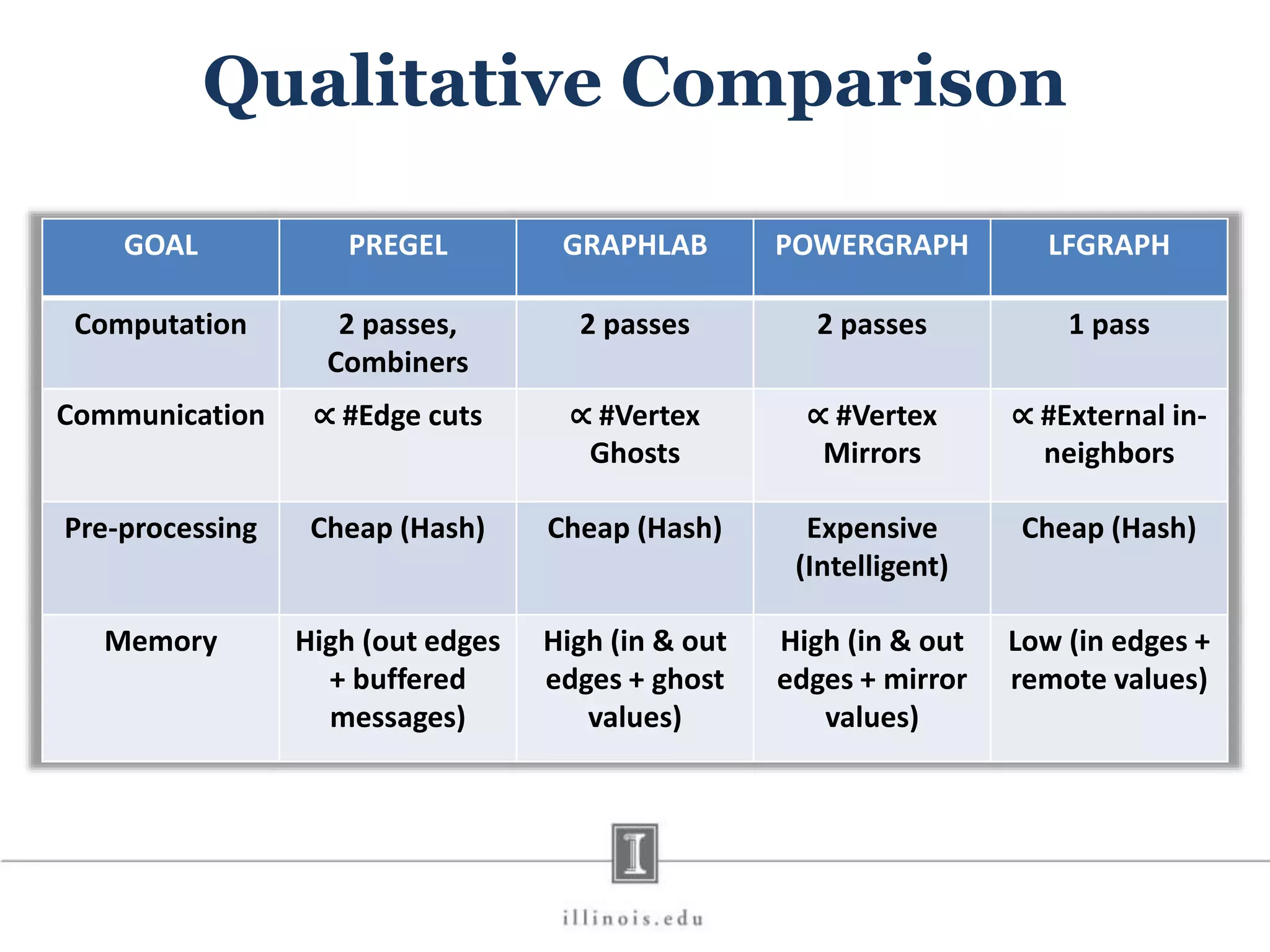
GRAPH PROCESSING
Why Graph Processing? Graphs are everywhere!
Why Graph Processing?
Why Distributed Graph Processing? They are getting bigger!
Road Scale >24 million vertices >58 million edges *Route Planning in Road Networks - 2008
Social Scale >1 billion vertices ~1 trillion edges *Facebook Engineering Blog ~41 million vertices >1.4 billion edges *Twitter Graph- 2010
Web Scale >50 billion vertices >1 trillion edges *NSA Big Graph Experiment- 2013
Brain Scale >100 billion vertices >100 trillion edges *NSA Big Graph Experiment- 2013
CHALLENGES IN PARALLEL GRAPH PROCESSING Lumsdaine, Andrew, et al. "Challenges in parallel graph processing." Parallel Processing Letters 17.01 -2007
Challenges 1 Structure driven computation Data Transfer Issues 2 Irregular Structure Partitioning Issues *Concept borrowed from Cristina Abad’s PhD defense slides
Overcoming the challenges 1 Extend Existing Paradigms 2 BUILD NEW FRAMEWORKS!
Build New Graph Frameworks! Key Requirements from Graph Processing Frameworks
1 Less pre-processing 2 Low and load-balanced computation 3 Low and load-balanced communication 4 Low memory footprint 5 Scalable wrt cluster size and graph size
PREGEL Malewicz, Grzegorz, et al. "Pregel: a system for large-scale graph processing.“ ACM SIGMOD -2010.
Life of a Vertex Program Placement Of Vertices Iteration 0 Iteration 1 Barrier Barrier Barrier Time Computation Communication *Concept borrowed from LFGraph Slides Computation Communication
B D C E A Sample Graph *Graph Borrowed from LFGraph Paper
B D C E A Shortest Path Example
B 0 D ∞ C ∞ E ∞ A ∞ Iteration 0
B 0 D ∞ C ∞ E ∞ A 1 Iteration 1
B 0 D 2 C ∞ E 2 A 1 Iteration 2
Can we do better? GOAL PREGEL Computation 1 Pass Communication ∝ #Edge cuts Pre-processing Cheap (Hash) Memory High (out edges + buffered messages)
LFGRAPH – YES, WE CAN! Hoque, Imranul, and Indranil Gupta. "LFGraph: Simple and Fast Distributed Graph Analytics”. TRIOS-2013
B D C E A Features Cheap Vertex Placement: Hash Based Low graph initialization time
B D C E A Features Publish Subscribe fetch once information flow Low communication overhead
B D C E A Subscribe Subscribing to vertex A
B D C E A Publish Publish List of Server 1: (Server2, A)
B D C E A LFGraph Model Value of A
B D C E A Features Only stores in-neighbor vertices Reduces memory footprint
B D C E A In-neighbor storage Local in-neighbor – simply read the value Remote in-neighbor – read locally available value
B 0 D ∞ C ∞ E ∞ A ∞ Iteration 0
B 0 D ∞ C ∞ E ∞ A ∞ Iteration 1 A 1 Value change in duplicate store Value of A
B 0 D ∞ C ∞ E ∞ A 1 Iteration 2 Local read of A Local read of A D 2 E 2
B D C E A Features Single Pass Computation Low computation overhead
Life of a Vertex Program Placement Of Vertices Iteration 0 Iteration 1 Barrier Barrier Barrier Time Computation Communication Computation Communication *Concept Borrowed from LFGraph Slides
How everything Works
GRAPHLAB Low, Yucheng, et al. "Graphlab: A new framework for parallel machine learning”. Conference on Uncertainty in Artificial Intelligence (UAI) - 2010
B D C E A A D E GraphLab Model
Can we do better? GOAL GRAPHLAB Computation 2 passes Communication ∝ #Vertex Ghosts Pre-processing Cheap (Hash) Memory High (in & out edges + ghost values)
POWERGRAPH Gonzalez, Joseph E., et al. "Powergraph: Distributed graph-parallel computation on natural graphs." USENIX OSDI - 2012.
B D C E A1 A2 PowerGraph Model
Can we do better? GOAL POWERGRAPH Computation 2 passes Communication ∝ #Vertex Mirrors Pre-processing Expensive (Intelligent) Memory High (in & out edges + mirror values)
Communication Analysis External on edge cuts Ghost vertices - in and out neighbors Mirrors - in and out neighbors External in neighbors
Computation Balance Analysis • Power Law graphs have substantial load imbalance. • Power law graphs have degree d with probability proportional to d-α. •Lower α means a denser graph with more high degree vertices.
Computation Balance Analysis
Real World vs Power Law
Communication Balance Analysis
PageRank – Runtime w/o partition
PageRank – Runtime with partition
PageRank – Memory footprint
PageRank – Network Communication
Scalability
X-Stream: Edge-centric Graph Processing using Streaming Partitions * Some figures adopted from author’s presentation
Motivation • Can sequential access be used instead of random access?! • Can large graph processing be done on a single machine?!
Sequential Access: Key to Performance! Medium Read (MB/s) Write (MB/s) Random Sequential Speed up Random Sequential Speed up RAM (1 core) 567 2605 4.6 1057 2248 2.2 RAM (16 core) 14198 25658 1.9 10044 13384 1.4 SSD 22.5 667.69 29.7 48.6 576.5 11.9 Magnetic Disk 0.6 328 546.7 2 316.3 158.2 Speed up of sequential access over random access in different media Test bed: 64 GB RAM + 200 GB SSD + 3TB drive
How to Use Sequential Access? Sequential access … Edge-Centric Processing
Vertex-Centric Scatter for each vertex v if state has updated for each output edge e of v scatter update on e
Vertex-Centric Gather for each vertex v for each input edge e of v if e has an update apply update on state
1 6 3 5 8 7 4 2 BFS SOURCE DEST 1 3 1 5 2 7 2 4 3 2 3 8 4 3 4 7 4 8 5 6 6 1 8 5 8 6 V 1 2 3 4 5 6 7 8 Vertex-Centric
Edge-Centric Scatter for each edge e if e.source has updated scatter update on e A B C = Updated Vertex Update u1 Update un
Edge-Centric Gather for each update u on edge e apply update u to e.destination X Y Z = Updated Vertex Update u1 Update un Update u2 X Y Z
Sequential Access via Edge-Centric! In Fast Storage In Slow Storage In Slow Storage
Fast and Slow Storage
1 6 3 5 8 7 4 2 SOURCE DEST 1 3 1 5 2 7 2 4 3 2 3 8 4 3 4 7 4 8 5 6 6 1 8 5 8 6 V 1 2 3 4 5 6 7 8 BFS Edge-Centric Lots of wasted reads! Most real world graphs have small diameter Large Diameter makes X-Stream slow and wasteful
SOURCE DEST 1 3 1 5 2 7 2 4 3 2 3 8 4 3 4 7 4 8 5 6 6 1 8 5 8 6 66 = SOURCE DEST 1 3 8 6 5 6 2 4 3 2 4 7 4 3 3 8 4 8 2 7 6 1 8 5 1 5 Order is not important No pre-processing (sorting and indexing) needed!
But, still … • Random access for vertices • Vertices may not fit into fast storage
Streaming Partitions V=Subset of vertices E=Outgoing edges of V U=Incoming updates to V Mutually disjoint Changing in each scatter phase Constant set
Vn En Un Scatter and Shuffle V1 E1 U1 Input buffere1 e2 e3 … Update bufferu1 u2 u3 … Output bufferu'1 u'2 u'3 … Vertex setv1 v2 v3 … Fast Memory Read source Add update Shuffle … Append to updates
Shuffle Stream Buffer with k partitions
Gather V1 E1 U1 Update bufferu1 u2 u3 … Vertex setv1 v2 v3 … Fast Memory Apply update No output!
Parallelism • State stored in vertices • Disjoint vertex set in partitions Compute partitions in parallel Parallel scatter and gather
Experimental Results
X-Stream Speedup over Graphchi 0 1 2 3 4 5 6 Netflix/ALS Twitter/Pagerank Twitter/Belief Propagation RMAT27/WCC Mean Speedup = 2.3 Speedup without considering the pre-process time of Graphchi
0 1 2 3 4 5 6 Netflix/ALS Twitter/Pagerank Twitter/Belief Propagation RMAT27/WCC X-Stream Speedup over Graphchi Mean Speedup = 3.7 Speedup considering the pre-process time of Graphchi
0 500 1000 1500 2000 2500 3000 Time(sec) Graphchi Sharding X-Stream runtime X-Stream Runtime vs Graphchi Sharding
Disk Transfer Rates Metric X-Stream Graphchi Data moved 224 GB 322 GB Time taken 398 seconds 2613 seconds Transfer rate 578 MB/s 126 MB/s 77 SSD sustain reads = 667 MB/s, writes = 576 MB/s Data transfer rates on Page Rank algorithm on Twitter workload
Scalability on Input Data size 0:00:01 0:00:05 0:00:21 0:01:24 0:05:37 0:22:30 1:30:00 6:00:00 24:00:00 Time(HH:MM:SS) RAM SSD Disk 8 Million V, 128 Million E, 8 sec 256 Million V, 4 Billion E, 33 mins 4 Billion V, 64 Billion E, 26 hours
Discussion • Features like global values, aggregation functions, asynchronous computation missing from LFGraph. Will the overhead of adding these features slow it down? • LFGraph assumes that all edge values are same. If the edge values are not, either the receiving vertices or the server will have to incorporate that value. Overheads? • LFGraph has one pass computation but then it executes the vertex program at each vertex (active or inactive). Trade-off?
Discussion • Independent computation and communication rounds may not always be preferred. Use bandwidth when available. • Faul Tolerance is another feature missing from LFGraph. Overheads? • Three benchmarks for experiments. Enough evaluation? • Scalability comparison with Pregel with different experiment settings. Memory comparison with PowerGraph based on heap values from logs. Fair experiments?
Discussion • Could the system become asynchronous? • Could the scatter and gather phase be combined into one phase? • Does not support iterating over the edges/updates of a vertex. Can this be added? • How good do they determine number of partitions? • Can shuffle be optimized by counting the updates of each partition during scatter?
Thank you for listening! Questions?
Backup Slides
Reason for Improvement
Qualitative Comparison GOAL PREGEL GRAPHLAB POWERGRAPH LFGRAPH Computation 2 passes, Combiners 2 passes 2 passes 1 pass Communication ∝ #Edge cuts ∝ #Vertex Ghosts ∝ #Vertex Mirrors ∝ #External in- neighbors Pre-processing Cheap (Hash) Cheap (Hash) Expensive (Intelligent) Cheap (Hash) Memory High (out edges + buffered messages) High (in & out edges + ghost values) High (in & out edges + mirror values) Low (in edges + remote values)
Backup Slides
Read Bandwidth - SSD 0 200 400 600 800 1000 Read(MB/s) 5 minute window X-Stream Graphchi
Write Bandwidth - SSD 0 100 200 300 400 500 600 700 800 Write(MB/s) 5 minute window X-Stream Graphchi
Scalability on Thread Count
Scalability on Number of I/O Devices
Sharding-Computing Breakdown in Graphchi 0 0.1 0.2 0.3 0.4 0.5 0.6 0.7 0.8 0.9 1 FractionofRuntime Benchmark Graphchi Runtime Breakdown Compute + I/O Re-sort shard
X-Stream not Always Perfect
Large Diameter makes X-stream Slow!
In-Memory X-Stream Performance 0 50 100 1 2 4 8 16 Runtime(s)Loweris better Threads BFS (32M vertices/256M edges) BFS-1 [HPC 2010] BFS-2 [PACT 2011] X-Stream
Ligra vs. X-Stream
Discussion • The current implementation is on a single machine, can it be extended to clusters? – Would it still perform good – How to provide fault tolerance and synchronization? • The waste rate is high (~65%). Could this be improved? • Can the partition be more intelligent? Dynamic partitioning? • Could all vertex-centric programs be converted to edge-centric? • When does streaming outperform random access?

Graph processing

Editor's Notes

  • #2 Hi, I am Mayank and the second presenter for today is Shadi. We will be talking about Graph Processing.
  • #3 Let’s start from the very basic question. Why do we need graph processing? The answer is simple and I am sure all of you already know. Graphs are everywhere! We have the web, indexed web used by search engines, social networks-Facebook, Twitter, road networks and biological networks like brain networks, spread of disease networks, graphs representing relationship between genomic sequences and so on.
  • #4 Let’s start from the very basic question. Why do we need graph processing? The answer is simple and I am sure all of you already know. Graphs are everywhere! We have the web, indexed web used by search engines, social networks-Facebook, Twitter, road networks and biological networks like brain networks, spread of disease networks, graphs representing relationship between genomic sequences and so on.
  • #5 Another simple question is why do we need distributed graph processing? Because these graphs are getting bigger! Let me give you an idea of the scale that we are talking about!
  • #6 Starting from the scale of road networks About 24 million vertices and 58 million edges in the US road network
  • #7 The social scale is bigger with about a billion vertices and nearly trillion edges
  • #8 The web scale is even bigger with an estimated 50 billion vertices
  • #9 However, the biggest scale is the brain network scale with over 100 billion vertices and 100 trillion edges. Moving on to the challenges that arise in parallel graph processing when dealing with such large scale graphs.
  • #10 Now, MapReduce is a very popular framework for batch processing of data. A natural question came up-why not simply use MapReduce for parallel graph processing. The framework will handle distribution and fault tolerance, speculative execution and all and everything will be perfect. But, there are some unique properties of graphs that makes using MapReduce harder or lets say expensive and that paradigm is not a perfect match for graph processing. I will be talking briefly about this paper published in the Parallel Processing Letters highlighting both software and hardware challenges for parallel graph processing. Remember, I am giving a brief history about how graph processing ahs evolved over the years. I will discuss only the software challenges here. Some of them also highlight why MapReduce is not a perfect fit for graph processing.
  • #11 The first is that graph computations are data-driven in the sense that they incorporate the graph structure into the computations. This gives rise to two issues: It is not clear how the graph should be partitioned across the machines (Remember with MapReduce-partitioning files is easy) Since, graph processing involves computation over the graph structure, these frameworks will incur a high overhead in the resultant data transfer. If it is not clear how data transfer comes into the picture more with graphs, it will become clear once I move onto how graphs are actually processed. The next challenge is that graph data is irregular. Real world graphs like social graphs are Power law like graphs (The reason why I say power law like and not power law will also become clear in this presentation). What this means that there are some vertices with high degrees while others with low degrees. This irregularity gives rise to two concerns: It is not clear how partitioning should be performed – some vertices require more processing while others require less – how do you incorporate this into MapReduce. Scalability of a MapReduce cluster will take a hit due to difficulty in achieving a good load balancing. The next challenge is achieving locality with graph processing. Since the data is irregular, it is difficult to predict the access patterns of vertices – which vertex will be processed when, which vertex will require more data to be fetched over the network, how do you take these issues into account in MapReduce.
  • #12 Now, what possible solutions did the community come up with. The solutions proposed can be classified into two broad categories: Extend MapReduce and make changes to solve these challenges Come up with novel paradigms and frameworks. This talk is mainly about the second solution but let me give you just a brief example of how the community tried to shoehorn graph processing in MapReduce.
  • #13 Moving on to the second approach i.e. coming up with paradigms/frameworks that handle graph processing by themselves. Paradigms designed just for graph processing. Before I discuss graph processing frameworks, what are the key requirements from these frameworks.
  • #14 First Depends on number and distribution of vertices and edges across servers Second depends on quantity and distribution of data exchanged among vertices across servers Third for quick initialization of the graph
  • #15 This started with Google coming up with a vertex centric form of computation called Pregel. The idea is simple – you have to think like a vertex.
  • #16 Think like a vertex If you visualize how graph processing works – there is some computation done at the vertex which passes along the computation results along the edges. I will explain this with an example. Let us first look at the life of a vertex centric program. The entire computation is broken down into iterations/supersteps. In each iteration, there is a computation phase and a communication phase. During the computation phase, the vertices perform computation and during the communication phase, they transfer the results of the computation to their neighbors. More concretely, In each superstep, a vertex receives messages sent to the vertex in superstep S-1, performs some computation in a user defined function compute() and sends messages to either its neighbors or any other vertex with a known identifier (these messages are received in superstep S+1) But the core idea is that the programmer should just have to worry about what each vertex does and the framework does the rest itself. The framework will ensure that these vertex programs are executed parallely and the messages are delivered to the right vertices. Fault tolerance is also handled by the framework, things like speculative execution of a vertex program are handled. Overlapping computation and communication
  • #17 Let us take the example if single source shortest paths to make this clear. This is a sample graph with five vertices – All edge weights are same and equal to 1. Each vertex has an id and a value. The value denotes the shortest path distance to source. In superstep 0, no messages received. The value is either initialized to 0 (if vertex is source) or MAX (otherwise) and advertized to neighbors In other supersteps, the vertex determines the minimum value of all the messages received. If this minimum is smaller than the value that the vertex currently holds, the value is updated and advertized to neighbors
  • #18 The aim is to compute the distance from a single source – in this case B. Initially, all vertices have this distance as infinity.
  • #19 In iteration zero, each vertex checks if it is the source. If it is, it makes its value 0. Otherwise, the value remains infinity. If the value of a vertex changes, it forwards the value plus the edge value along all outgoing edges. In this case, B sends a message with value 1 towards A.
  • #20 In the next iteration, A simply takes the minimum of values received in the messages (minimum because only the minimum value matters). If the minimum is smaller than the value that the vertex already had, it makes its value as that smaller value. In this case, A makes its value 1. Since, there was a change in its value. It propagates the change to its neighbours. If you all haven’t already guessed – this is basically breadth first search happening iteratively.
  • #21 This continues till no more values change.
  • #22 What was the problem with this simple yet powerful paradigm? The main problem is that vertices communicate with each other. Hence, A sends its values to both D and E even though they are on the same server. Pregel provides an abstraction called combiners where all messages being sent to a particular vertex from the same server are combined. For example, in the single source shortest paths case, the vertex does not need to receive all messages, it just needs to receive the message which has the smallest value. Combiners do this. However, they need an additional pass over messages.
  • #23 So came LFGraph with the aim of minimizing the three requirements memory, computation and communication.
  • #24 Next feature that I have already touched upon is the cheap hash based initial vertex placement. This reduces the time required for the initialization of the graph.
  • #25 Moving on to the four main features of LFGraph that helps it achieve superior performance as compared to the exisiting frameworks. The first is the fetch once behavior achieved using the publish subscribe lists. Server 2 needs to fetch the value of Vertex A only once and not the case like in Pregel where each vertex receives the value in a message.
  • #26 The first step is partitioning. LFGraph chooses to use a cheap partitioning strategy (unlike PowerGraph and GraphLab) that perform expensive initial vertex partitioning. We will see the benefits from this cheap initial partitioning in the experiments section. The cheal partitioning used is simple hashing. Next, servers subscribe for vertices. Server 2 realizes that its vertices need the value of vertex A so it communicates this to Server 1.
  • #27 Based on this communication, each server builds a publish list. For each server, values of which vertices need to be sent to that server. This is maintained for each server and at each server.
  • #28 Next, the vertex centric computations are performed on each server. And, at the end of the iteration, each server simply looks at the publish list and sends the values of vertices that each server needs. I did not discuss one important aspect of computation. When computation is performed, the values of vertices may change. This changed value is stored in one place while the original values are kept in another place. These two copies are required because a vertex may have edge to another vertex on the same server. For example, here the value of A may change during computation – so the vertices B and C should read the value that existed before the iteration started. The other way to do this is to lock the vertices. Locking is much more expensive than maintaining two copies. LFGraph opts for computation savings in this case at the cost of extra memory overhead. However, the authors show that the space overhead of keeping these values is not much.
  • #29 LFGraph needs to store only the in-neighbors. Out neighbors are not required since each vertex that has in neighbors on other servers uses the publish subscribe list to inform the server.
  • #30 The first step is partitioning. LFGraph chooses to use a cheap partitioning strategy (unlike PowerGraph and GraphLab) that perform expensive initial vertex partitioning. We will see the benefits from this cheap initial partitioning in the experiments section. The cheal partitioning used is simple hashing. Next, servers subscribe for vertices. Server 2 realizes that its vertices need the value of vertex A so it communicates this to Server 1.
  • #31 In iteration zero, each vertex checks if it is the source. If it is, it makes its value 0. Otherwise, the value remains infinity. If the value of a vertex changes, it forwards the value plus the edge value along all outgoing edges. In this case, B sends a message with value 1 towards A.
  • #32 In the next iteration, A simply takes the minimum of values received in the messages (minimum because only the minimum value matters). If the minimum is smaller than the value that the vertex already had, it makes its value as that smaller value. In this case, A makes its value 1. Since, there was a change in its value. It propagates the change to its neighbours. If you all haven’t already guessed – this is basically breadth first search happening iteratively.
  • #33 This continues till no more values change.
  • #34 The third feature is the single pass computation. The framework just makes one pass over the vertices during the computation phase. An additional pass is obviously required in the communication phase. I hope I am clear about passes in computation. In each computation phase, the framework needs to go through the list of vertices and execute the vertex centric program once for each vertex.
  • #35 Think like a vertex Unlike Pregel, decouples computation and communication – independent growth of each other. If you visualize how graph processing works – there is some computation done at the vertex which passes along the computation results along the edges. I will explain this with an example. Let us first look at the life of a vertex centric program. The entire computation is broken down into iterations/supersteps. In each iteration, there is a computation phase and a communication phase. During the computation phase, the vertices perform computation and during the communication phase, they transfer the results of the computation to their neighbors. More concretely, In each superstep, a vertex receives messages sent to the vertex in superstep S-1, performs some computation in a user defined function compute() and sends messages to either its neighbors or any other vertex with a known identifier (these messages are received in superstep S+1) But the core idea is that the programmer should just have to worry about what each vertex does and the framework does the rest itself. The framework will ensure that these vertex programs are executed parallely and the messages are delivered to the right vertices. Fault tolerance is also handled by the framework, things like speculative execution of a vertex program are handled.
  • #36 Explain this?
  • #37 Front End servers: Store vertex program and configuration file (regarding graph data, number of servers, ips, ports, number of computation and communication job servers etc) It sends the vertex program and configuration file to all the servers Graph Loaders load the graph parallely across servers and store it in storage engine Each server then enters the barrier Barrier waits for all servers to enter and then signals them to continue Job Server spawns multiple workers to compute on a part of the graph – shard Job Server enters barrier at the end of all worker thread completion After signal from Barrier Server, communication phase just like computation phase And repeat
  • #39 Next came GraphLab. The idea here is to create ghost vertices. The idea is to have zero communication within an iteration. Ghost vertices are created for vertices that have an edge from a vertex on another server. In this example- A has an edge to D and E. So a ghost vertices D and E is created on Server 1. Similarly, a ghost vertex is created for vertex A on Server 2. All the values that the vertices on each server need are present with the server. However, if the value of D changes after an iteration, it needs to be communicated to all its ghost vertices. In this example, if the value of A changes on server 1 in iteration s, that new value will be communicated to server 2 after iteration s and before iteration s+1.
  • #40 The communication overhead here is proportional to the number of ghosts. Additionally, the servers need to store both in and out vertices to handle the ghost vertices. Also, there is a 2 pass computation with one pass for value updates and one for neighbor activation (i.e. determine if a vertex needs to perform any computation – performs computation only if it has an active neighbor/ i.e. it is receiving a message)
  • #42 Next came PowerGraph, the idea here is mirrors. Instead of creating ghost vertices, the vertices which have edges on multiple servers have mirrors on all the servers. For example, the vertex A creates two mirrors – one on Server 1 and another on Server 2. Now, just like ghost vertices, the values of mirrors need to be accumulated. It assigns a master mirror that collects all values and sends the final value to all mirrors.
  • #43 Therefore, here the communication overhead is twice the number of mirrors. All these are excellent approaches but can we do better? The problem is that there are three major requirements from a graph framework – low memory overhead, low computation overhead and low communication overhead. But all of them do not go hand in hand. Can we minimize each in a single framework. The frameworks that we discussed till now trade one for another. I will discuss the comparison between all the frameworks in a later slide.
  • #44 The authors used the equations that they derived to calculate the expected communication overhead as the number of servers increases for real world graphs. This is Twitter. LFGraph is better than all. But one interesting observation is that LFGraph is still increasing at 250 while Pregel plateaus. No matter how many servers, the probability of having neighbors on other servers is uniform
  • #45 I mentioned before that Cheap hash based partitioning is better than expensive intelligent partitioning. Let us discuss exactly why this is the case. It has been shown in several studies that Power Law graphs have substantial load imbalance if we use a random hash based partitioning. People have used this to motivate the need for an intelligent partitioning strategy up front to reduce the imbalance. Remember that more the imbalance more is the execution time. Since there are barriers, each iteration is only as fast as the slowest worker. However, are real world graphs same as ideal power law graphs.
  • #46 The runtime of a computation worker during an iteration is proportional to the total number of in edges processed by that worker If we use synthetic ideal power law graphs, it is true the imbalance is high.
  • #47 However, if we use real world graphs, the imbalance is low. So whats the difference between power law graphs and real world graphs.
  • #48 While ideal power-law graphs have a straight tail in their log-log plot, each of the real graphs has a funnel at its tail. This indicates that in real graphs there are lots of the highest degree vertices – so they spread out and become load-balanced across servers, because the servers are far fewer in number than vertices. On the other hand, in an idealized power-law graph, there is only one of the very highest degree vertex and this causes unbalanced load.
  • #49 If we plot the total number of vertices fetched during the communication phases, we observe very little imbalance across the workers showing that communication is balanced in LFGraph.
  • #50 Random – randomly place edges across machines Batch (greedy partitioning without global coordination) – In a greedy manner, place the next edge on the machine that minimizes the number of mirrors /replication factor - with global co-ordination using a global table Oblivious (greedy partitioning with global coordination) – Each machine locally decides – no global coordination LFGraph is 2x faster than the best PowerGraph variant
  • #51 In a small cluster with 8 servers, LFGraph is between 4x to 100x faster than the PowerGraph variants. In a large cluster with 32 servers the improvement grows to 5x–380x. We observed that PowerGraph’s intelligent partitioning schemes contributed 90% –99% to the overall runtime for the PageRank benchmark. In a small cluster, distributed graph processing is compute-heavy thus intelligent partitioning (e.g., in PowerGraph) has little effect. In a large cluster, intelligent partitioning can speed up iterations – however, the partitioning cost itself is directly proportional to cluster size and contributes sizably to runtime.
  • #52 Used smem tool to measure memory footprint for LFGraph Heap Space reported in the Debug Logs to estimate memory footprint LFGraph uses 8x to 12x less memory than PowerGraph.
  • #53 LFGraph transfers about 4x less data per server than PowerGraph As the cluster size is increased, there is first a quick rise in the total communication overhead (see Section 4 and Figure 3). Thus the per-server overhead rises at first. However as the total communication overhead plateaus out, the cluster size increase takes over, thus dropping the per-server overhead. This creates the peak in between. *Emulab has full-bisection badwidth
  • #54 We create 10 synthetic graphs vary ing in number of vertices from 100M to 1B, and with up to 128B edges. We run the SSSP benchmark on it. mu =4 and sigma =1.3 However, different numbers of servers for Pregel and LFGraph and different configurations on these servers 300 servers with 800 workers vs 12 servers with 96 workers
  • #56 Sequential access by far faster than random access.
  • #57 Sequential access beats random access for every medium Increasing performance for slower media Even in ram faster because of pre fetching! Random write better than read: RAM: write coalescing buffers in the architecture of the used RAM Write cache on disk ( absorbing writes, letting next write to be done while the previous is outstanding) Why 16 less than 1? We need to use 16 to saturate the memory Why increasing for slower media? Of their architectur moving head is expensive, ram is designed for random access
  • #59 State stored in vertices Scatter updates along outgoing edge Gather updates from incoming edges
  • #60 State stored in vertices Scatter updates along outgoing edge Gather updates from incoming edges
  • #62 State stored in vertices Scatter updates along outgoing edge Gather updates from incoming edges
  • #63 State stored in vertices Scatter updates along outgoing edge Gather updates from incoming edges Scatter and gather in a loop until termination criterion is met When edge set >> vertex set the benefit of streaming rather than accessing randomly increases
  • #64 Streaming data from slow storage
  • #66 Wasted edges!
  • #67 No index No clustering No sorting
  • #69 Union of Vs must create all vertices V must fit in fast storage  The number of partition is important for the performance  3 streaming files
  • #70 They have an extra in and out buffer for streaming
  • #71 Static allocation! Create index array Copy updates to partition chunks
  • #75 Why some less?? Higher waste -> either the algorithm it self or bigger diameter Wcc: weakly connected components Belief propagation: Pagerank: Als alternating Least Squares Graphchi uses “shards” Partitions edges into sorted shards First to bring notion of sequential access V and in/out edges of the shard need to be in memory at the same time!  more shards! Needs pre sorting( based on src) , are resorting of updates X-Stream uses sequential scans Partitions edges into unsorted streaming partitions Without pre sorting time
  • #76 Mainly bacuse of re-sorting ( to destination)60% Incomplete use of available streaming bandwidg from ssd ( more shardes fits edges as well)
  • #77 X-Stream returns answers before Graphchi finishes sharding In 3/4
  • #78  X-Stream uses all available bandwidth from the storage device
  • #79 Weakly connected components Log-log -> linear linear Unordere graph -> easily ahndles bigger graphs 330M edges added at time WCC Why 3 out of 16?
  • #82 In partitions number they assume uniform distribution of updates. How realistic? In traversal algorithms?
  • #85 In LFGraph, computation and communication phases are independent. Independent growth of each phase + Communication can be batched In PowerGraph, the two phases overlap ->Communication negatively impacts computation
  • #86 Here is the table given in the paper pointing out the qualitative comparison between various frameworks. As you can see, LFGraph achieves the minimum overheads across the categories. I will not spend time on the table too much but it is clear.
  • #88 Gather-> all read . No write-> write=0 Scatter -> bursty Sequential access bandwidth Graphchi shard All vertices and edges must fit in memory X-Stream partition Only vertices must fit in memory More Graphchi shards than X-Stream partitions Makes access more random for Graphchi
  • #90 Wcc bfs traversal
  • #91 HDD RMAT:30 SSD RMAT:27 Take advantage of extra disk!
  • #94 Ratio of execution to streaming
  • #95 Less difeernce since more cores -> differnce random decreases
  • #96 Pre processing only once, used many times! Xstrema not always the best especially traversal algoritms ( high waste) Pre 7-8x more than xstream
  • #97 There is waste reads with streaming, but streaming is faster than random access. When to choose which? If more edges -> more random access  makes slower, but more wastage at the same time Intelligent partition: try to put vertices that have the same output vertex set together try to have same edge list size of the set for load balancing dynamic can cause a high overhead This would cause overhead, and we want low overhead!