Download to read offline
![The Boston house-price data has been used in many machine learning papers that address regression problems. Tools used: Pandas Numpy Matplotlib scikit-learn Python Implementation with code : Import necessary libraries Import the necessary modules from specific libraries. import numpy as np import pandas as pd %matplotlib inline import matplotlib.pyplot as plt from sklearn.model_selection import train_test_split from sklearn import datasets from sklearn.metrics import mean_squared_error from sklearn import ensemble Load the data set Use the pandas module to read the taxi data from the file system. Check few records of the dataset. # ############################################################################# # Load data boston = datasets.load_boston() print(boston.data.shape, boston.target.shape) print(boston.feature_names) (506, 13) (506,) ['CRIM' 'ZN' 'INDUS' 'CHAS' 'NOX' 'RM' 'AGE' 'DIS' 'RAD' 'TAX' 'PTRATIO' 'B' 'LSTAT'] data = pd.DataFrame(boston.data,columns=boston.feature_names) data = pd.concat([data,pd.Series(boston.target,name='MEDV')],axis=1) data.head() CRIM ZN INDUS CHAS NOX RM AGE DIS RAD TAX PTRATIO B LSTAT MEDV 0 0.00632 18.0 2.31 0.0 0.538 6.575 65.2 4.0900 1.0 296.0 15.3 396.90 4.98 24.0 1 0.02731 0.0 7.07 0.0 0.469 6.421 78.9 4.9671 2.0 242.0 17.8 396.90 9.14 21.6 2 0.02729 0.0 7.07 0.0 0.469 7.185 61.1 4.9671 2.0 242.0 17.8 392.83 4.03 34.7 - MEDV Median value of owner-occupied homes in $1000's :Missing Attribute Values: None :Creator: Harrison, D. and Rubinfeld, D.L. This is a copy of UCI ML housing dataset. http://archive.ics.uci.edu/ml/datasets/Housing This dataset was taken from the StatLib library which is maintained at Carnegie Mellon University. The Boston house-price data of Harrison, D. and Rubinfeld, D.L. 'Hedonic prices and the demand for clean air', J. Environ. Economics & Management, vol.5, 81-102, 1978. Used in Belsley, Kuh & Welsch, 'Regression diagnostics ...', Wiley, 1980. N.B. Various transformations are used in the table on pages 244-261 of the latter.](https://image.slidesharecdn.com/gradientboostingforregressionproblemswithexamplebasicsofregressionalgorithm-181005085252/75/Gradient-boosting-for-regression-problems-with-example-basics-of-regression-algorithm-3-2048.jpg)
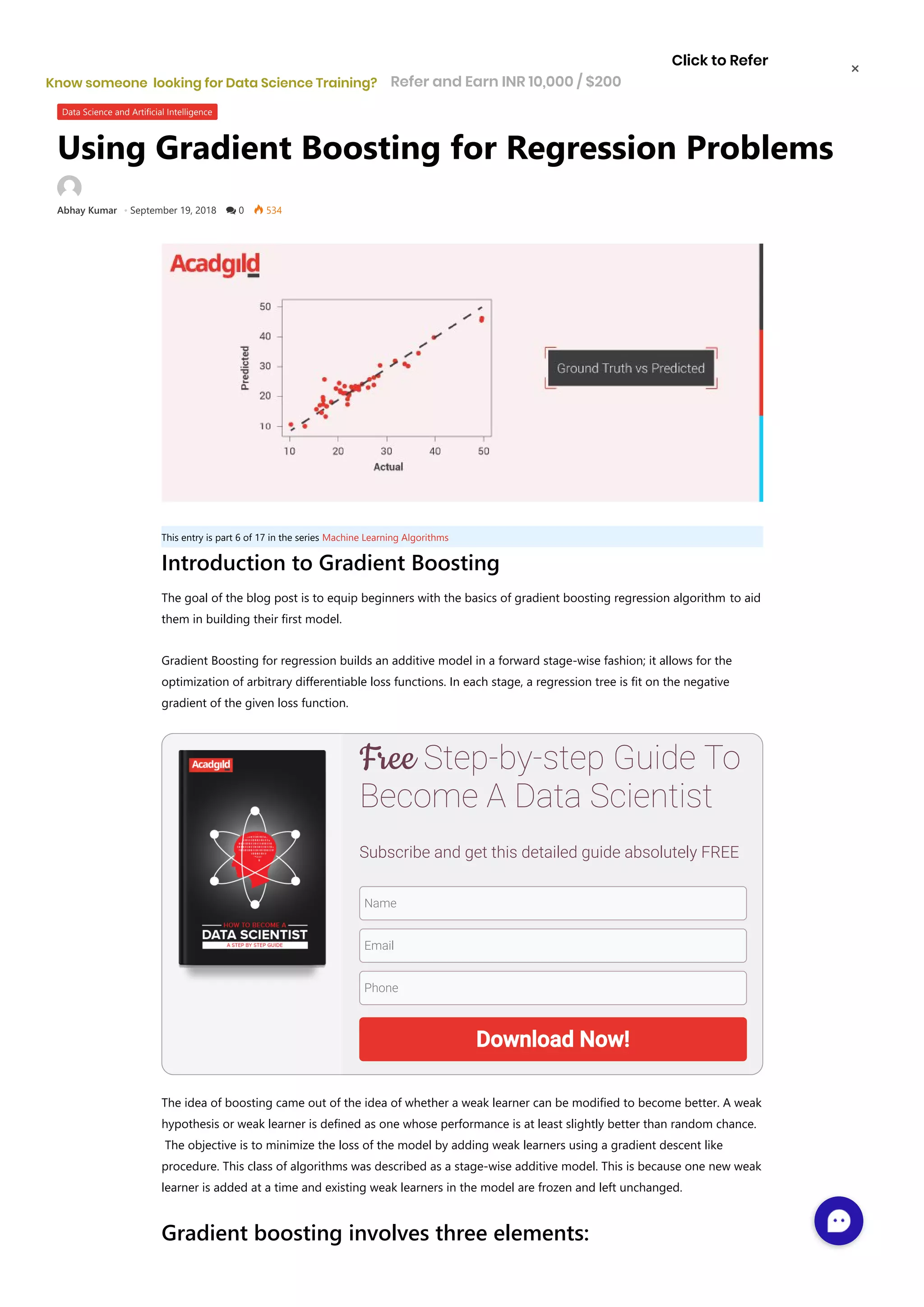
![3 0.03237 0.0 2.18 0.0 0.458 6.998 45.8 6.0622 3.0 222.0 18.7 394.63 2.94 33.4 4 0.06905 0.0 2.18 0.0 0.458 7.147 54.2 6.0622 3.0 222.0 18.7 396.90 5.33 36.2 Select the predictor and target variables X = data.iloc[:,:-1] y = data.iloc[:,-1] Train test split: x_training_set, x_test_set, y_training_set, y_test_set = train_test_split(X,y,test_size=0.10, random_state=42, shuffle=True) Training/model fitting: Fit the model to selected supervised data # Fit regression model params = {'n_estimators': 500, 'max_depth': 4, 'min_samples_split': 2, 'learning_rate': 0.01, 'loss': 'ls'} model = ensemble.GradientBoostingRegressor(**params) model.fit(x_training_set, y_training_set) Model parameters study : from sklearn.metrics import mean_squared_error, r2_score model_score = model.score(x_training_set,y_training_set) # Have a look at R sq to give an idea of the fit , # Explained variance score: 1 is perfect prediction print('R2 sq: ',model_score) y_predicted = model.predict(x_test_set) # The mean squared error print("Mean squared error: %.2f"% mean_squared_error(y_test_set, y_predicted)) # Explained variance score: 1 is perfect prediction print('Test Variance score: %.2f' % r2_score(y_test_set, y_predicted)) R2 sq: 0.9798997042218072 Mean squared error: 5.83 Test Variance score: 0.91 Accuracy report with test data : Let’s visualize the goodness of the fit with the predictions being visualized by a line # So let's run the model against the test data from sklearn.model_selection import cross_val_predict fig, ax = plt.subplots() ax.scatter(y_test_set, y_predicted, edgecolors=(0, 0, 0)) ax.plot([y_test_set.min(), y_test_set.max()], [y_test_set.min(), y_test_set.max()], 'k--', lw=4) ax.set_xlabel('Actual') ax.set_ylabel('Predicted') ax.set_title("Ground Truth vs Predicted") plt.show()](https://image.slidesharecdn.com/gradientboostingforregressionproblemswithexamplebasicsofregressionalgorithm-181005085252/75/Gradient-boosting-for-regression-problems-with-example-basics-of-regression-algorithm-4-2048.jpg)
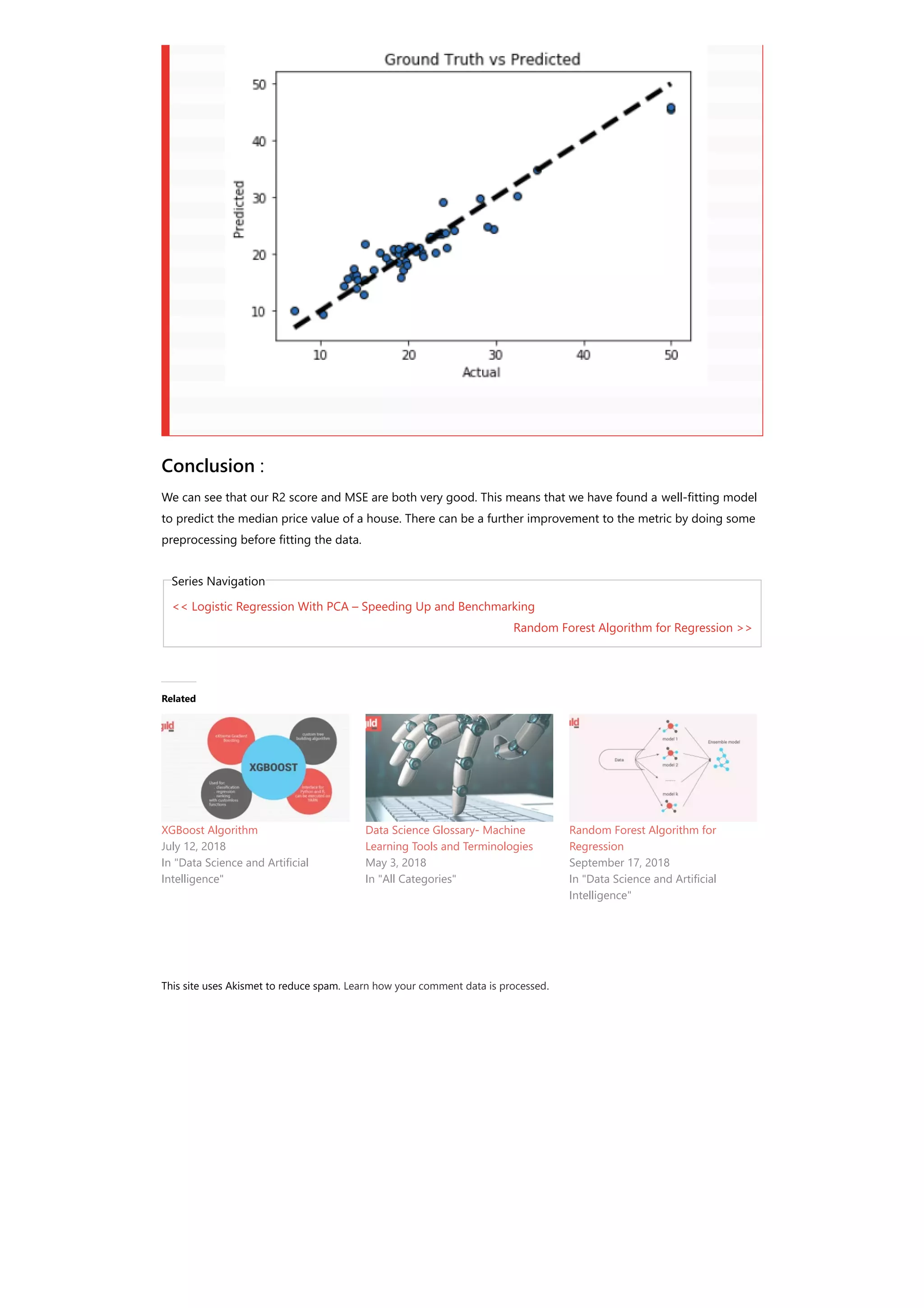

The document discusses using gradient boosting for regression problems. Gradient boosting builds an additive model in a stage-wise fashion to minimize a loss function. It uses decision trees as weak learners that are added sequentially. The document demonstrates implementing gradient boosting in Python to predict Boston housing prices based on various attributes. It loads the dataset, trains a gradient boosting regressor model on 80% of the data, and evaluates the model on the remaining 20% with metrics showing good performance.