Download as PDF, PPTX

![Dataset Preparation titanic<- read.csv("http://christianherta.de/lehre/dataScience/machine Learning/data/titanic-train.csv",header=T) sm_titantic_3<-titanic[,c(2,3,5,6,10)] #dont need all the columns sm_titanic_3<-sm_titantic_3[complete.cases(sm_titantic_3),] set.seed(43) tst_idx<-sample(714,200,replace=FALSE) tstdata<-sm_titanic_3[tst_idx,] trdata<-sm_titanic_3[-tst_idx,]](https://image.slidesharecdn.com/evaluatingclassifierperformance-ml-cs6923-161015001314/75/Evaluating-classifierperformance-ml-cs6923-3-2048.jpg)
![Running GLM Create a model using logistic regression glm_sm_titanic_3<-glm(Survived~.,data=trdata,family=binomial()) Predict using the test dataset and glm model created glm_predicted<- predict(glm_sm_titanic_3,tstdata[,2:5],type="response");](https://image.slidesharecdn.com/evaluatingclassifierperformance-ml-cs6923-161015001314/75/Evaluating-classifierperformance-ml-cs6923-4-2048.jpg)
![Calculate glm_sm_titanic_3<-glm(Survived~.,data=trdata,family=binomial()) glm_predicted<-predict(glm_sm_titanic_3,tstdata[,2:5],type="response"); require(ROCR) glm_auc_1<-prediction(glm_predicted,tstdata$Survived) glm_prf<-performance(glm_auc_1, measure="tpr", x.measure="fpr") glm_slot_fp<-slot(glm_auc_1,"fp") glm_slot_tp<-slot(glm_auc_1,"tp") Model with training and Predict with test Extract fp and tp using ROCR package glm_fpr3<-unlist(glm_slot_fp)/unlist(slot(glm_auc_1,"n.neg")) glm_tpr3<-unlist(glm_slot_tp)/unlist(slot(glm_auc_1,"n.pos")) Calculate fpr and tpr vectors glm_perf_AUC=performance(glm_auc_1,"auc") glm_AUC=glm_perf_AUC@y.values[[1]] Calculate Area Under Curve – ROC](https://image.slidesharecdn.com/evaluatingclassifierperformance-ml-cs6923-161015001314/75/Evaluating-classifierperformance-ml-cs6923-7-2048.jpg)
![Let us repeat the steps for individual trees tree<-rpart(Survived~.,data=trdata) tree_predicted_prob_03<- predict(pruned.tree.03,tstdata[,2:5]); tree_predicted_class_03<-round(tree_predicted_prob_03) tree_prediction_rocr_03<-prediction(tree_predicted_class_03,tstdata$Survived) tree_prf_rocr_03<-performance(tree_prediction_rocr_03, measure="tpr", x.measure="fpr") tree_perf_AUC_03= performance(tree_prediction_rocr_03,"auc") Model with training and Predict with test Extract measures using ROCR package plot(tree_prf_rocr_03,main="ROC plot cp=0.03(DTREE using rpart)") text(0.5,0.5,paste("AUC=",format(tree_perf_AUC_03@y.values[[1]],digits=5, scientific=FALSE))) #Use prune and printcp/plotcp to fine tune the model # as shown in the video We will use recursive partition package – there are many other packages Visualize](https://image.slidesharecdn.com/evaluatingclassifierperformance-ml-cs6923-161015001314/75/Evaluating-classifierperformance-ml-cs6923-9-2048.jpg)
![Let us repeat the steps for individual trees fac.titanic.rf<-randomForest(as.factor(Survived)~.,data=trdata,keep.inbag=TRUE, type=classification,importance=TRUE,keep.forest=TRUE,ntree=193) predicted.rf <- predict(fac.titanic.rf, tstdata[,-1], type='response') confusionTable <- table(predicted.rf, tstdata[,1],dnn = c('Predicted','Observed')) table( predicted.rf==tstdata[,1]) pred.rf<-prediction(as.numeric(predicted.rf),as.numeric(tstdata[,1])) perf.rf<-performance(pred.rf,measure="tpr",x.measure="fpr") auc_rf<-performance(pred.rf,measure="auc") Model with training and Predict with test Extract measures using ROCR package plot(perf.rf, col=rainbow(7), main="ROC curve Titanic (Random Forest)", xlab="FPR", ylab="TPR") text(0.5,0.5,paste("AUC=",format(auc_rf@y.values[[1]],digits=5, scientific=FALSE))) #Use prune and printcp/plotcp to fine tune the model # as shown in the video We will use randomForest package (which uses CART)– there are many other packages Visualize](https://image.slidesharecdn.com/evaluatingclassifierperformance-ml-cs6923-161015001314/75/Evaluating-classifierperformance-ml-cs6923-11-2048.jpg)
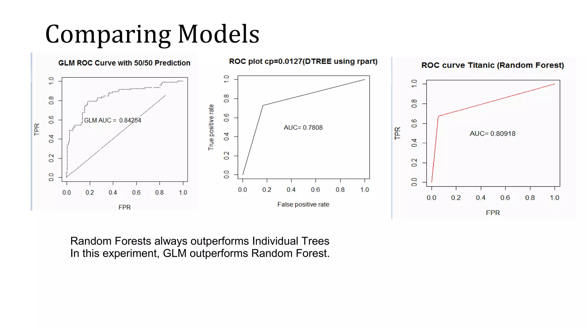
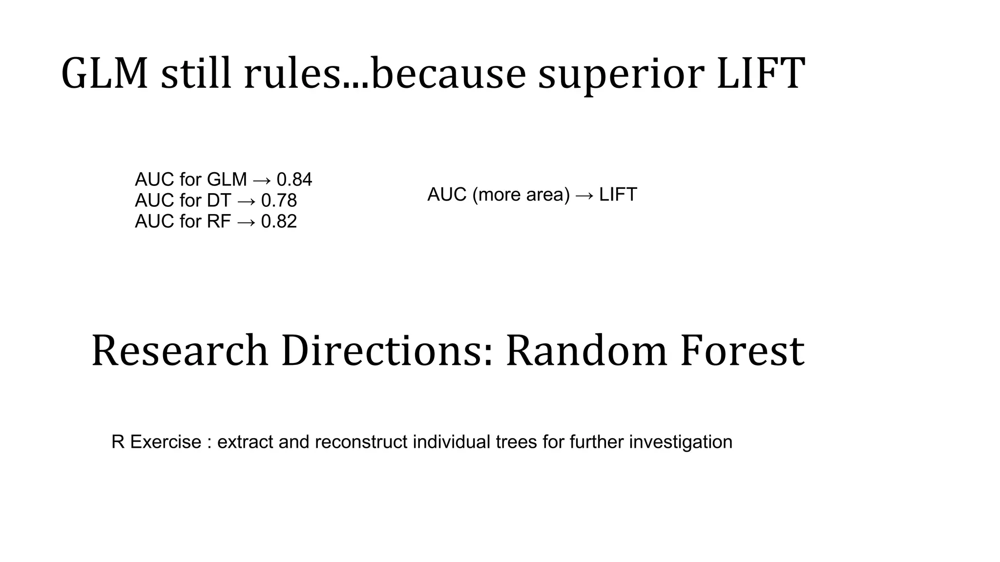

The document evaluates different classifier models for predicting Titanic survivor data: generalized linear models (GLM), decision trees, and random forests. It prepares training and test datasets and uses the ROCR package to calculate performance metrics like AUC for each model. GLM achieved the highest AUC of 0.84, outperforming the decision tree AUC of 0.78 and random forest AUC of 0.82. While random forests typically outperform individual trees, in this case GLM performed best due to its superior lift over other models.