The document presents a comparative analysis of various numerical methods for solving initial value problems in first order ordinary differential equations, focusing on Euler method, improved Euler method, and Runge-Kutta methods. It illustrates the accuracy of these methods by solving a standard first order differential equation and providing step-by-step calculations and results. The conclusion emphasizes that the fourth order Runge-Kutta method offers the most accurate and efficient solution among the methods compared.
![International Journal of Trend in Scientific Research and Development @ www.ijtsrd.com eISSN: 2456-6470 @ IJTSRD | Unique Paper ID – IJTSRD45066 | Volume – 5 | Issue – 5 | Jul-Aug 2021 Page 1342 with ⋅ ⋅ ⋅ ⋅ ⋅ = , 2 , 1 , 0 n whereh is step-size. Later on, Euler’s method is also known as first order Runge-Kutta method. The local error occurred in this method is proportional to the square of step size and the global error occurred in this method is proportional to step- size. 2. Improved Euler Method Euler method gives best result when the functions are linear in nature. When functions are non-linear there occurs a truncation error. To remove this drawback Improved Euler’s method is introduced. In this method instead of point the arithmetic average of the slopes at xn and xn+1(that is, at the end points of each subinterval) is used. This method based on two values of dependent variable 1 + n y and predicted value by Euler method i.e., 1 + n y . ( ) n n n n y x f h y y , 1 • + = + ( ) ( ) [ ] 1 1 1 , , 2 + + + + + = n n n n n n y x f y x f h y y This method is also known as Heun’s method or second order Runge-Kutta method. The local error occurred in this method is proportional to the cube of step size and the global error occurred in this method is proportional to square of step size. 3. Third order Runge-Kutta method The third order Runge-Kutta formula is as follows: ( ) ( ) ( ) 2 1 3 1 2 1 3 2 1 1 2 , 2 , 2 , 4 2 1 k k y h x f h k k y h x f h k y x f h k where k k k y y n n n n n n n n + − + • = + + • = • = + • + + = + This method is also known as Heun’s method of order Three. The local error occurred in this method is proportional to the fourth power of step size and the global error occurred in this method is proportional to cube of step size. 4. Fourth order Runge-Kutta method It is most popular Runge-Kutta method and widely used in solving the first order D.E. The formula for this method is as follows: ( ) ( ) ( ) 3 4 2 3 1 2 1 4 3 2 1 1 , 2 , 2 2 , 2 , 2 2 6 1 k y h x f h k k y h x f h k k y h x f h k y x f h k where k k k k y y n n n n n n n n n n + + • = + + • = + + • = • = + • + • + + = + The local error occurred in this method is proportional to the fifth power of step size and the global error occurred in this method is proportional to fourth power of step size. Application and comparison: Consider the first order ordinary D.E.as ( ) 1 0 , = − = y with y x dx dy . We first solve it by classical method and then by numerical methods. 1. Classical method: This is linear D.E. Comparing with ( ) ( ) x Q y x P dx dy = + Here ( ) ( ) x x Q x P = = , 1 Integrating factor= ( ) x dx dx x P e e e I = ∫ = ∫ = 1 It’s solution is ∫ + = c Idx Q I y c e xe ye x x x + − = Using initial conditions ( ) 1 0 = y 2 = c The particular solution is x e x y − + − = 2 1 For different values of x we get different solutions for y. Now we apply four above numerical method to given D.E. one by one. Here we consider the step size 0.2 for each method. The following table gives the value of y for x from 0 to 2, taking h=0.2.](https://image.slidesharecdn.com/178comparativeanalysisofdifferentnumericalmethods-210918050454/75/Comparative-Analysis-of-Different-Numerical-Methods-for-the-Solution-of-Initial-Value-Problems-in-First-Order-Ordinary-Differential-Equations-2-2048.jpg)
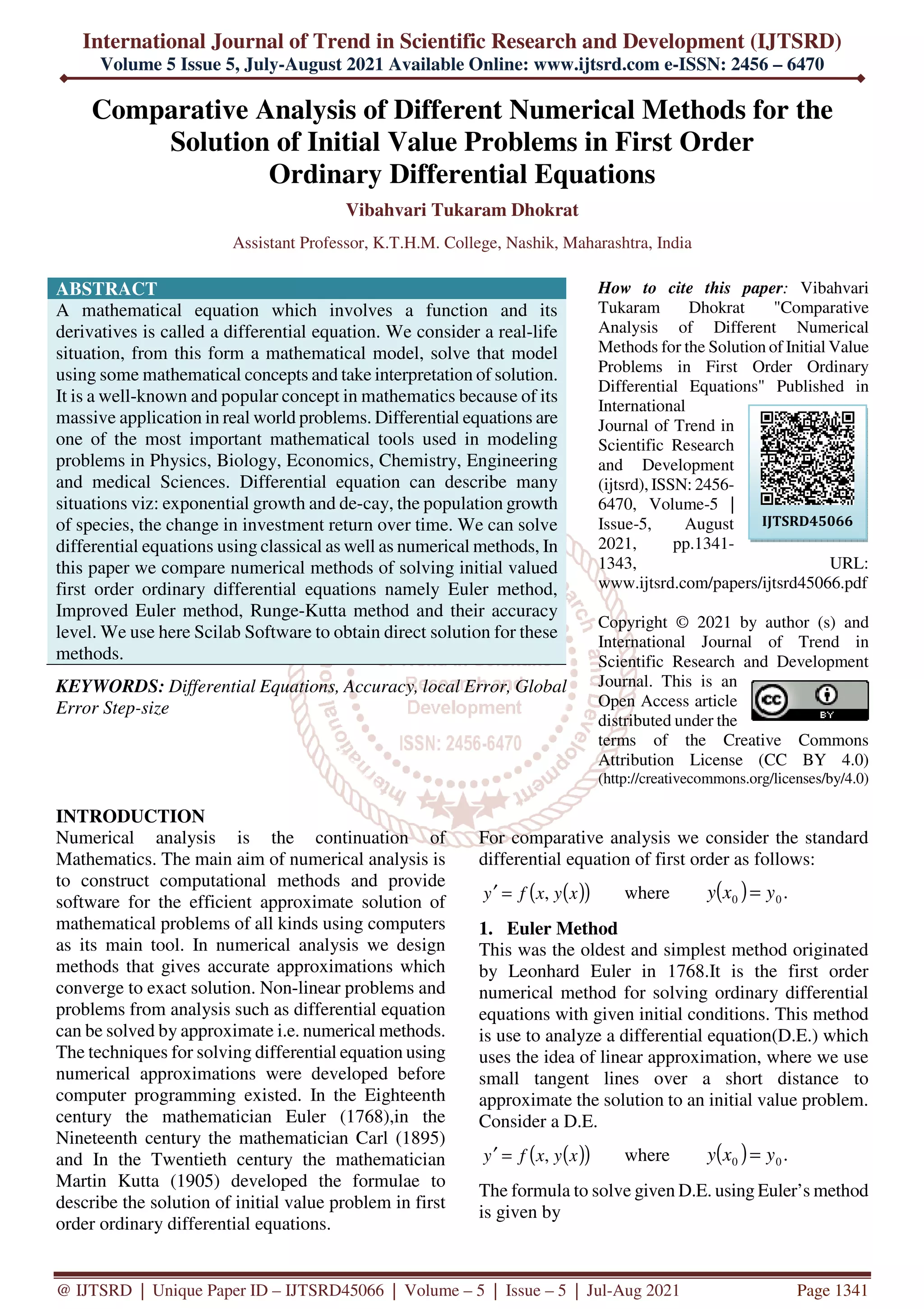
![International Journal of Trend in Scientific Research and Development @ www.ijtsrd.com eISSN: 2456-6470 @ IJTSRD | Unique Paper ID – IJTSRD45066 | Volume – 5 | Issue – 5 | Jul-Aug 2021 Page 1343 Sr. No. X Exact solution by classical method Euler’s method Improved Euler method Third order Runge- Kutta method Fourth order Runge- Kutta method 1 0 1 1 1 1 1 2 0.2 0.83746 0.80 0.84 0.82368 0.837467 3 0.4 0.74064 0.68 0.7448 0.721139 0.740649 4 0.6 0.69762 0.624 0.702736 0.677912 0.697634 5 0.8 0.69866 0.6192 0.704244 0.68237 0.698669 6 1 0.73576 0.65636 0.74148 0.725165 0.73577 7 1.2 0.80239 0.724288 0.808013 0.798781 0.8024 8 1.4 0.89319 0.8194304 0.898571 0.897175 0.893205 9 1.6 1.00379 0.9355443 1.00883 1.14982 1.0038 10 1.8 1.13060 1.0684355 1.13524 1.14982 1.13061 11 2 1.27067 1.2147484 1.2749 1.29702 1.27068 The above table shows that Euler’s method shows more variation with exact solution while Improved method and Fourth order Runge-kutta method gives solution which is closed to exact solution. Conclusion The main aim of this paper is to make the comparison between the numerical methods Euler method, Improved Euler method, Third order Runge-kutta method and Fourth order Runge-Kutta method and also with classical solution of first order ordinary D.E. In this paper we showed that the solution obtained by classical method is closed to solution obtained by numerical method. If in numerical method we reduce step size as small as possible to get more accurate solution. Among all these methods Fourth order Runge-kutta method gives more accurate and more efficient solution. Therefore, this method is widely used in solving first order ordinary D.E. References [1] Raisinghaniya, M.D., Ordinary and Partial Differential Equations, S. Chand&Comp. Ltd., 15th revised edition 2013,ISBN-81-219-0892-5. [2] S. S. Sastry., Introductory Methods of Numerical Analysis Fifth Edition, PHI Learning Private Limited, New-Delhi- 110001.2012. [3] Numerical Methods in Engineering with Python 3, Cambridge University Press 32 Avenue of the Americas, New York, NY 10013-2473, USA, ISBN 978-1-107-03385-6, 2013 [4] Scilab software. [5] Chapra, Steven C., & Canale Numerical Methods for Engineers, S Tata MacGraw Hill Education Pvt. L 25-902744-9. [6] Ince, E., L., Ordinary Differential Equations, First Edition, Dover Publication, Inc., New York. [7] Chandrajeet Singh Yadav, Comparative Analysis of Different Numerical Methods of Solving First Order Differential Equation., International Journal of Trend in Scientific Research and Development (ijtsrd), ISSN: 2456-6470, Volume-2, Issue-4, June 2018, pp.567-570,](https://image.slidesharecdn.com/178comparativeanalysisofdifferentnumericalmethods-210918050454/75/Comparative-Analysis-of-Different-Numerical-Methods-for-the-Solution-of-Initial-Value-Problems-in-First-Order-Ordinary-Differential-Equations-3-2048.jpg)