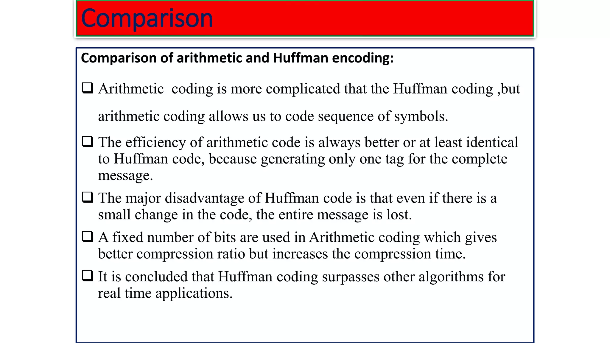
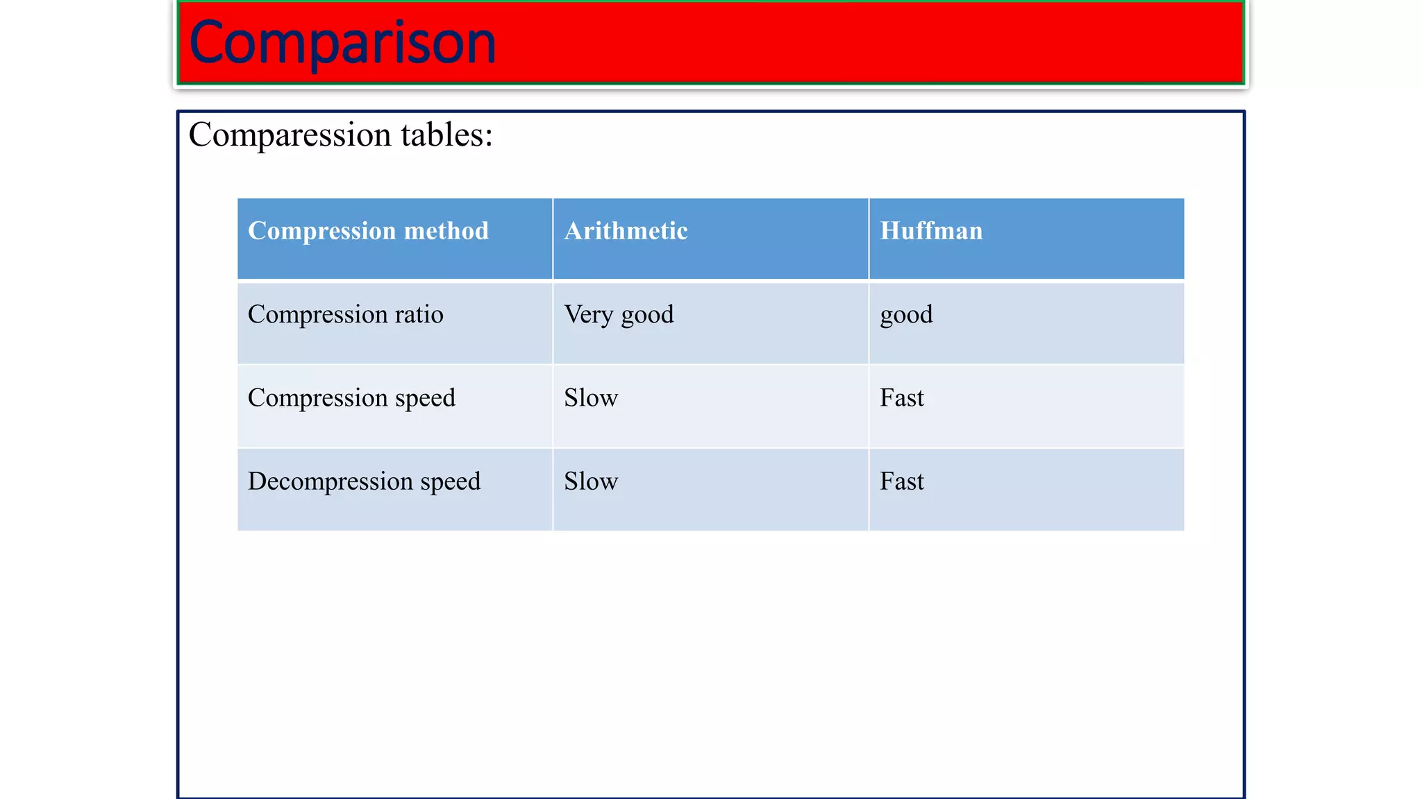
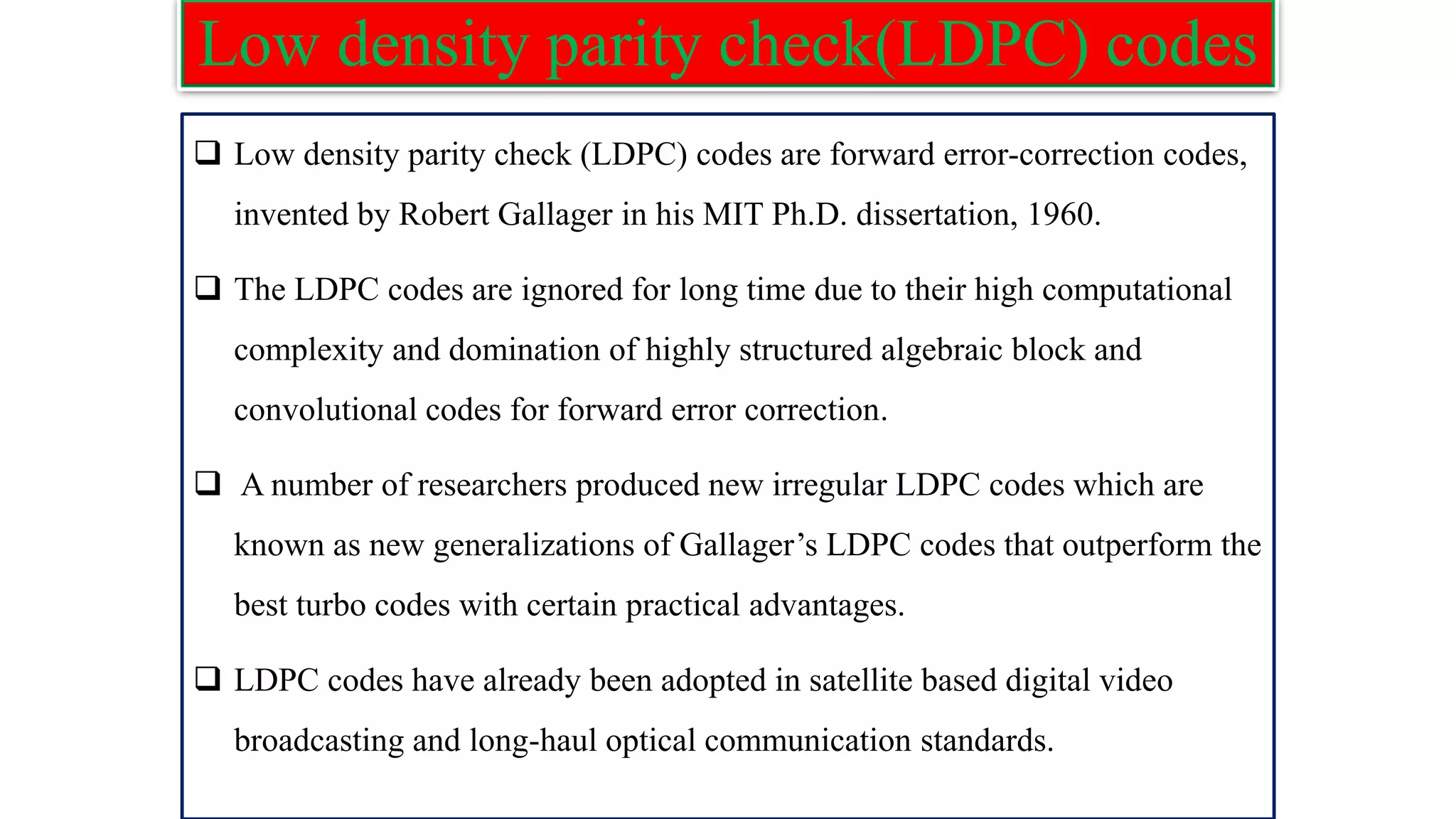
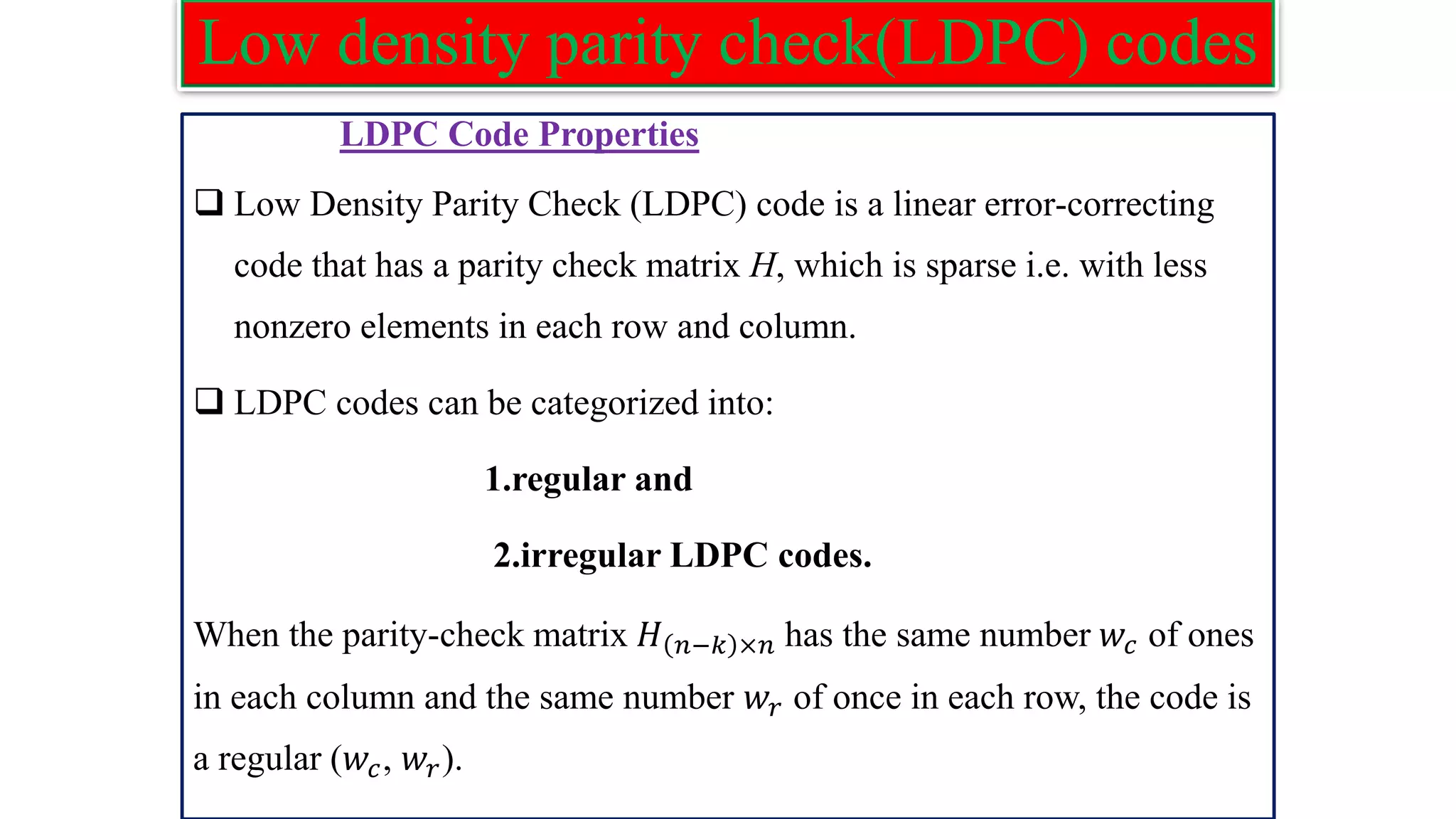
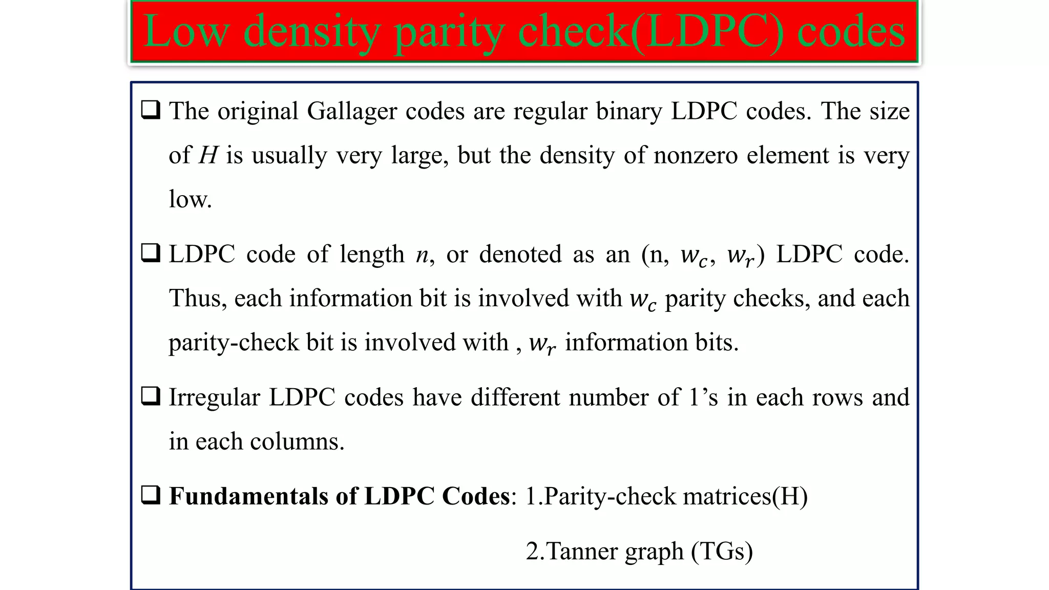
The document provides information on two coding techniques: arithmetic coding and low density parity check (LDPC) codes. It describes the algorithms, encoding process, and properties of arithmetic coding. It also introduces LDPC codes, discusses how their parity check matrices are constructed, and provides examples. The document compares arithmetic coding to Huffman coding and outlines some advantages and disadvantages of each approach.
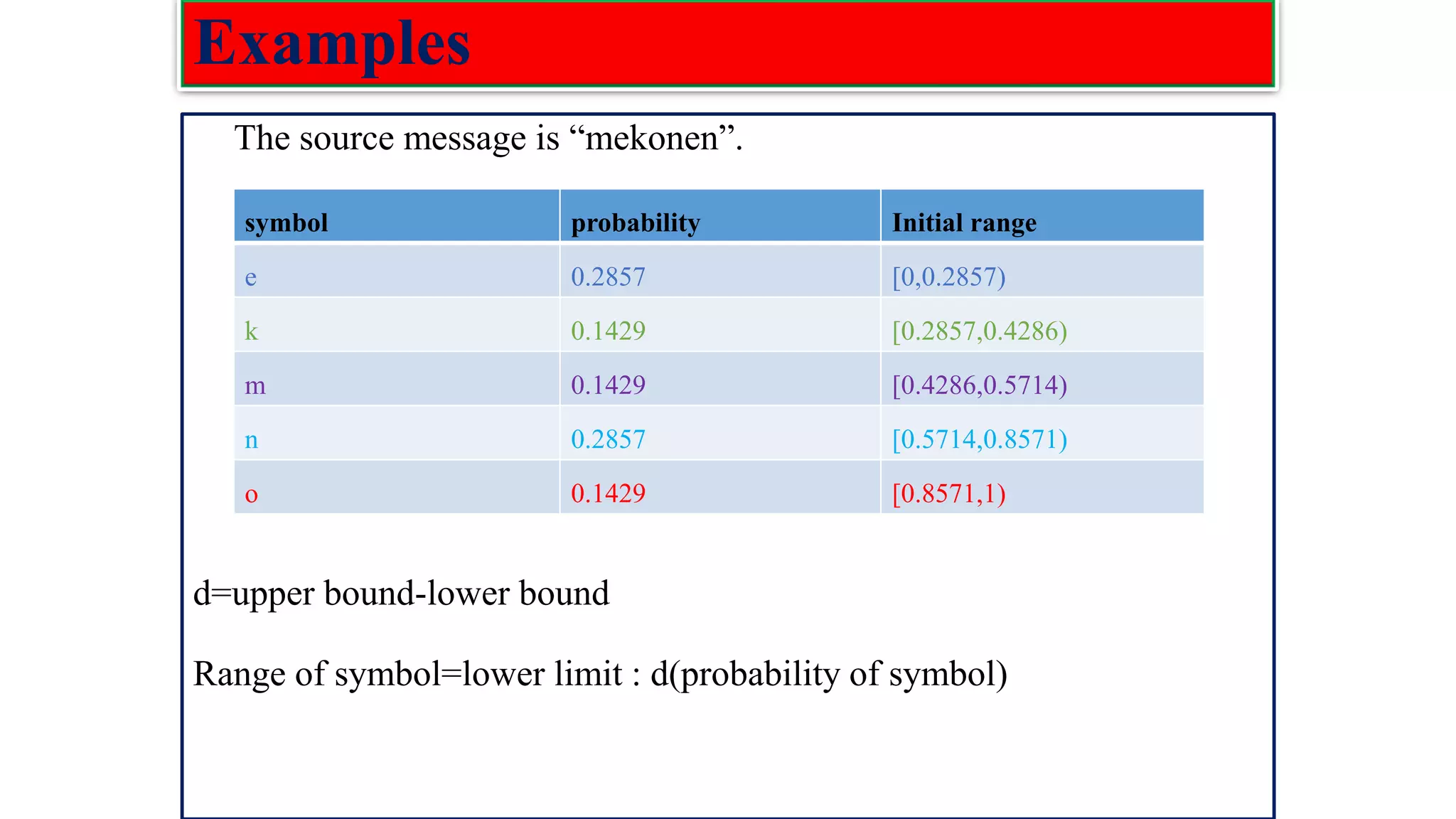
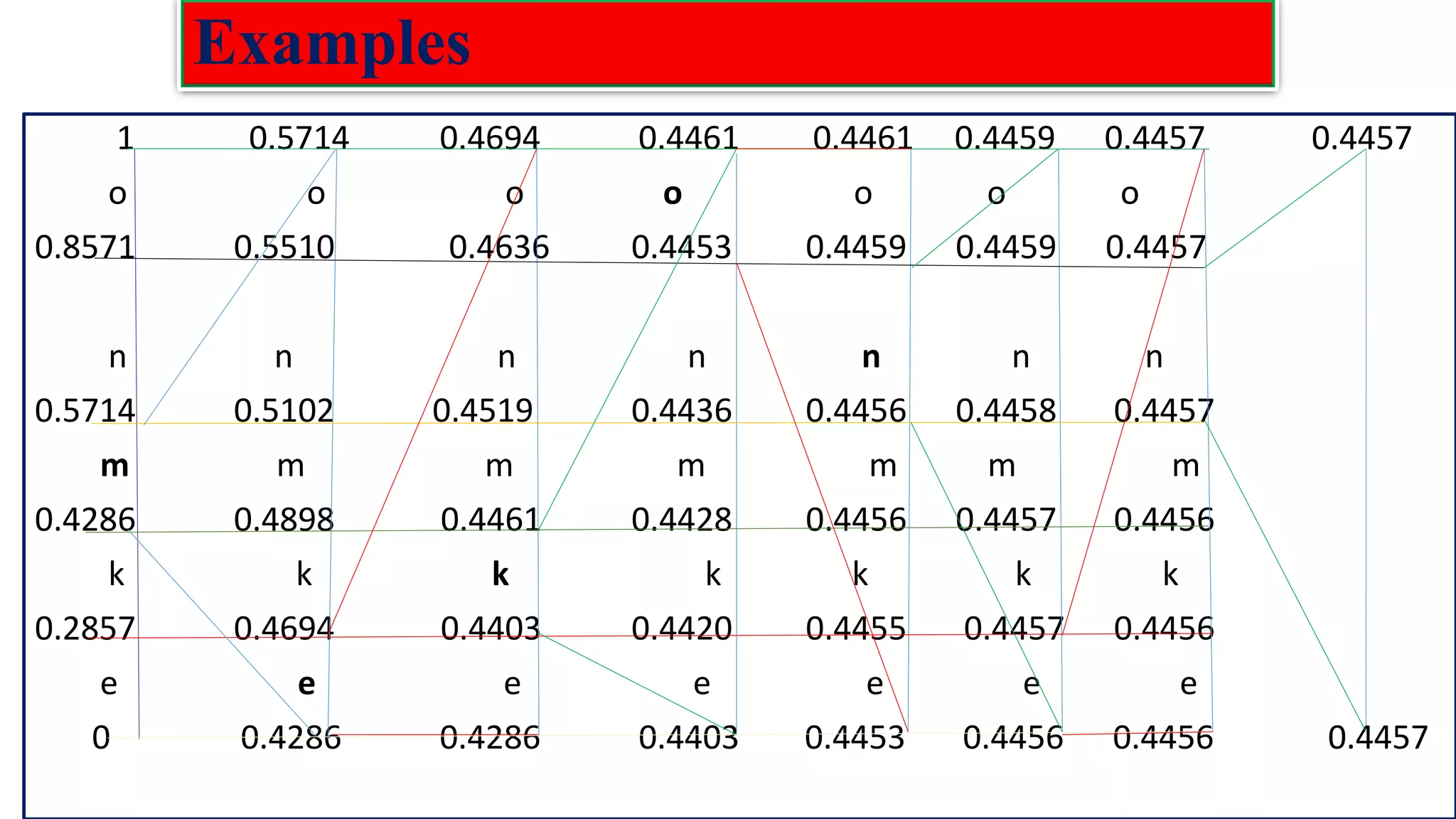
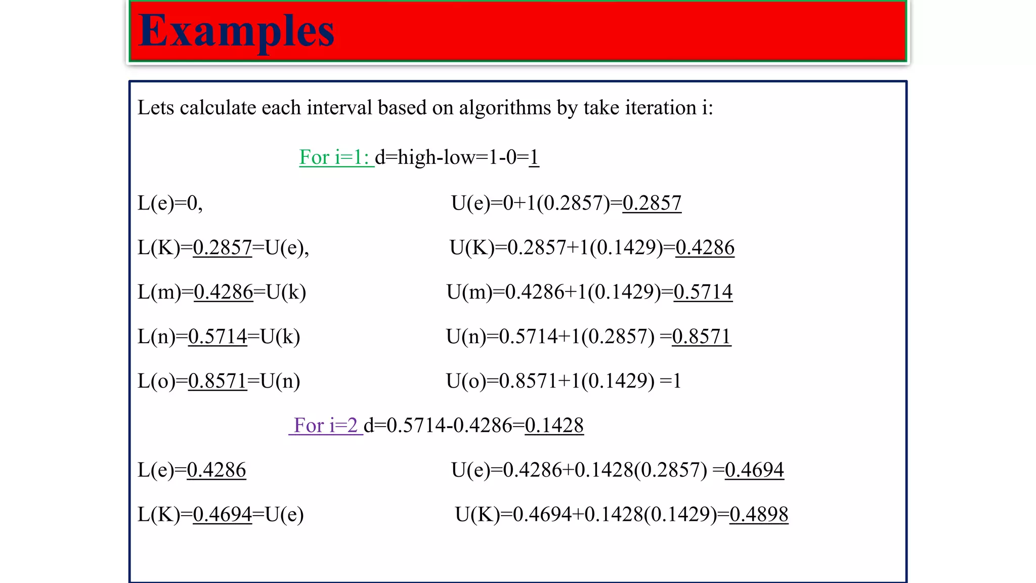
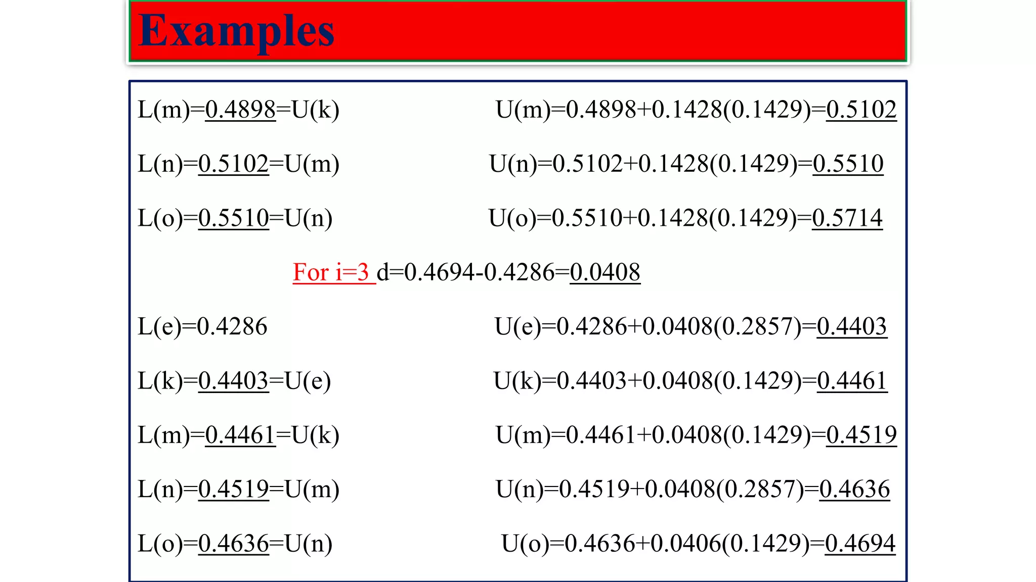
![Arithmetic coding ❑ In arithmetic coding a message is encoded as a number from the interval [0, 1). ❑ The number is found by expanding it according to the probability of the currently processed letter of the message being encoded. ❑ This is done by using a set of interval ranges IR determined by the probabilities of the information source as follows: IR={[0,𝑝1),[𝑝1,𝑝1+𝑝2),[ca𝑝1 + 𝑝2,𝑝1 + 𝑝2 + 𝑝3),…[𝑝1+…+𝑝𝑛−1, 𝑝1+…+𝑝𝑛)} Putting,𝑞𝑗 = σ𝑖=1 𝑗 𝑝𝑖, we n write IR ={[0,𝑞1),[𝑞1, 𝑞2),[𝑞𝑛−1,1) ❑ In arithmetic coding these subintervals also determine the proportional division of any other interval [L, R) contained in [0, 1) into subintervals 𝐼𝑅[𝐿,𝑅] as follows:](https://image.slidesharecdn.com/coding-230511112653-d56c6b69/75/coding-pdf-4-2048.jpg)
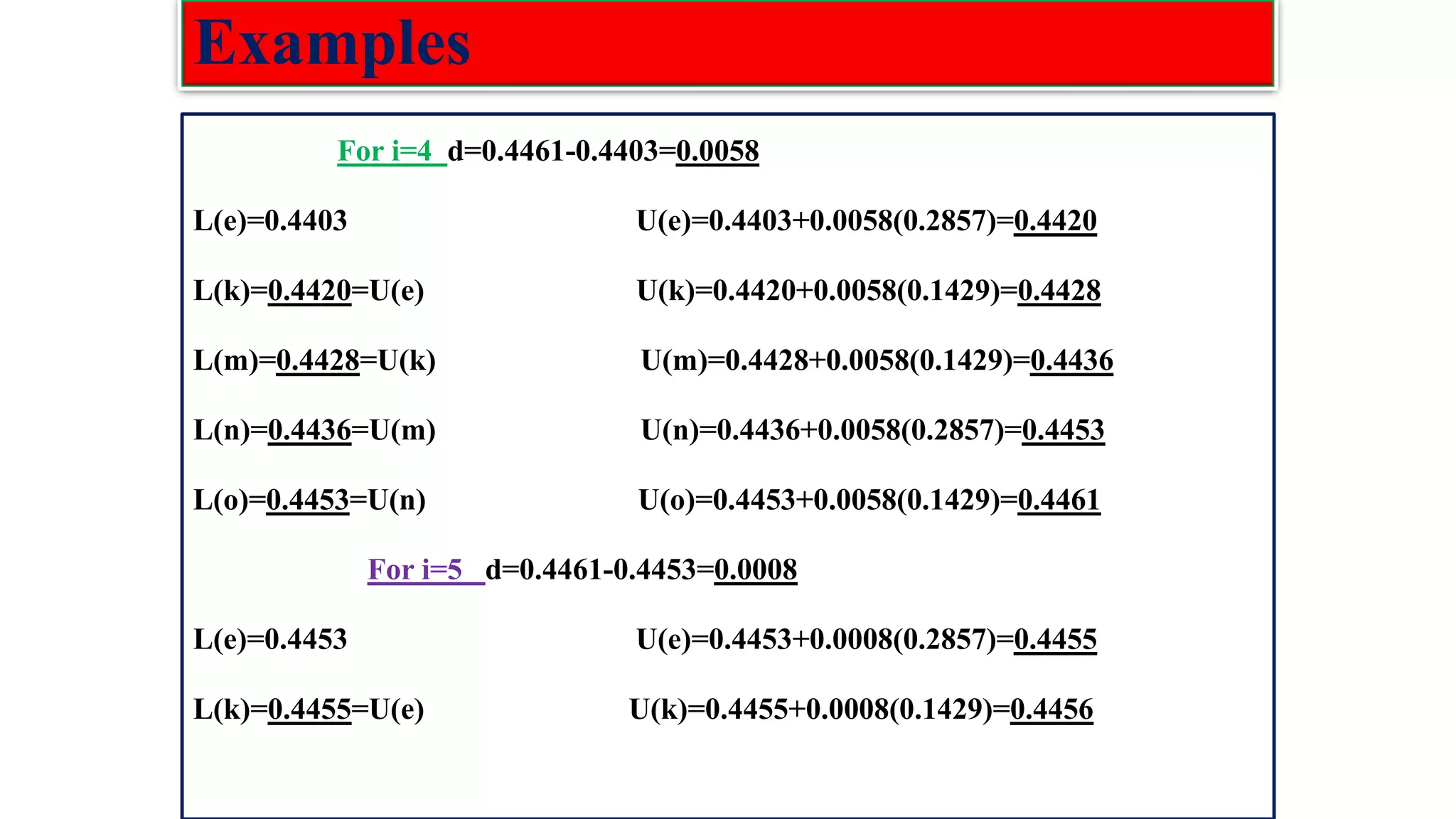
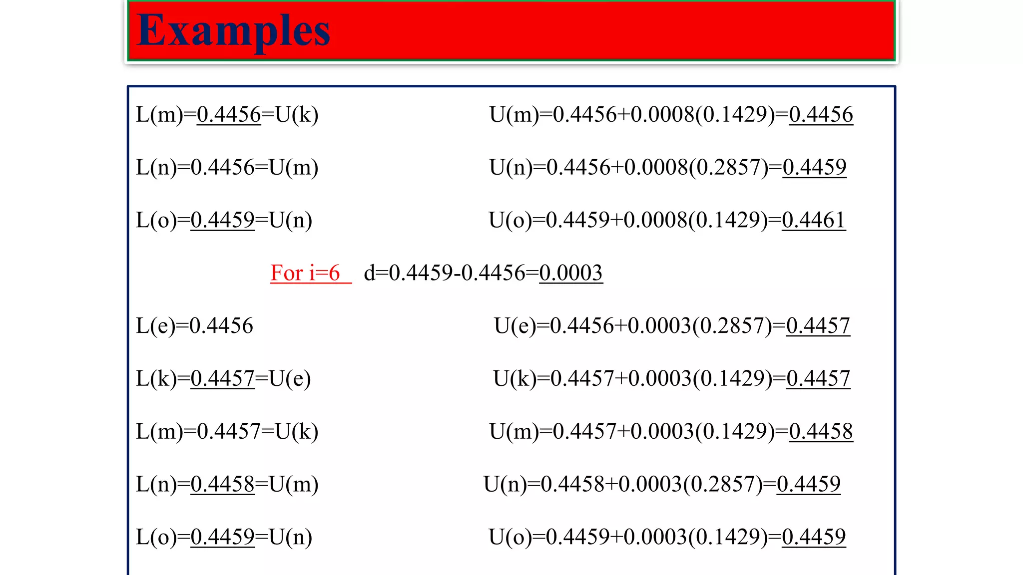
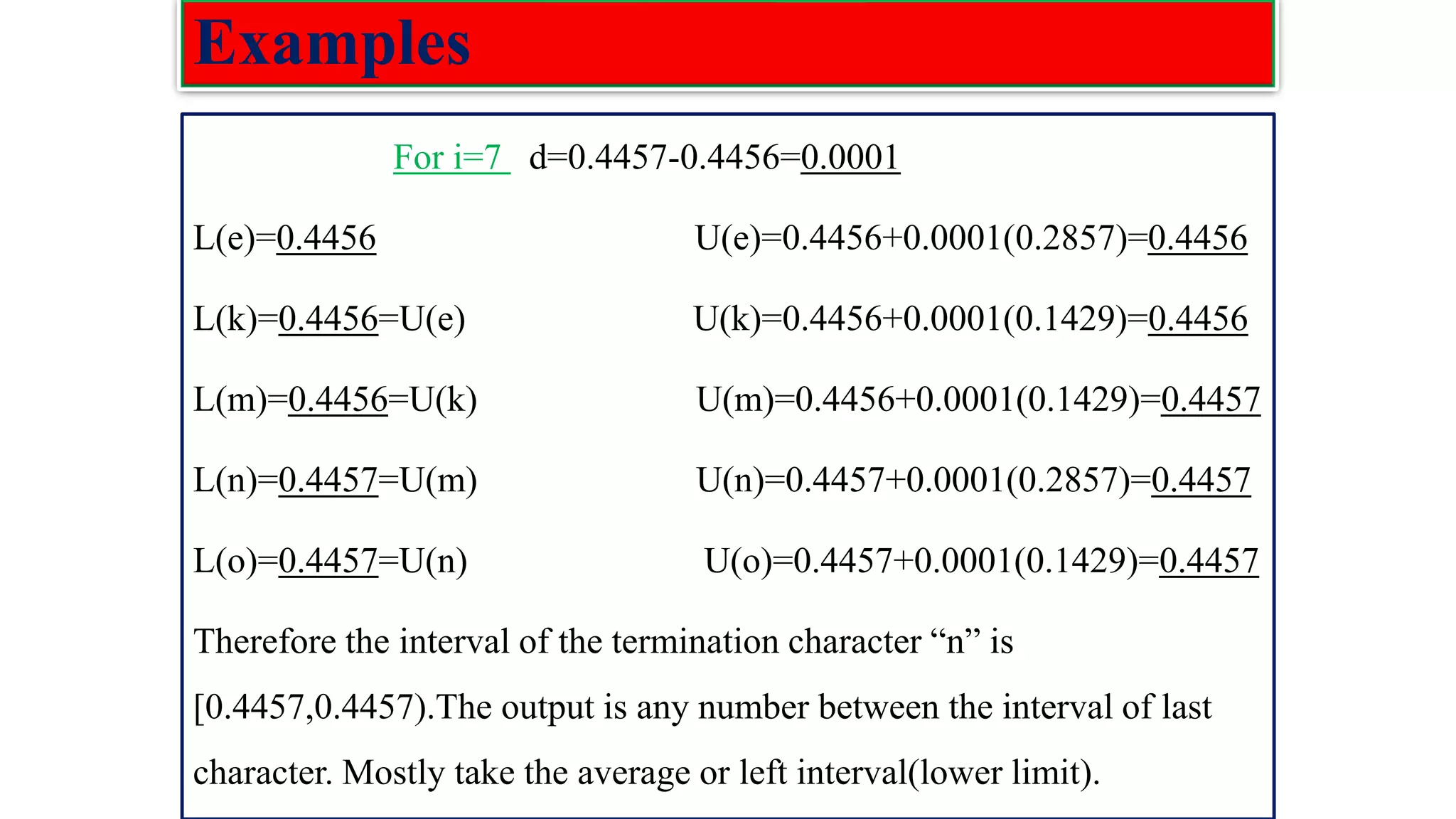
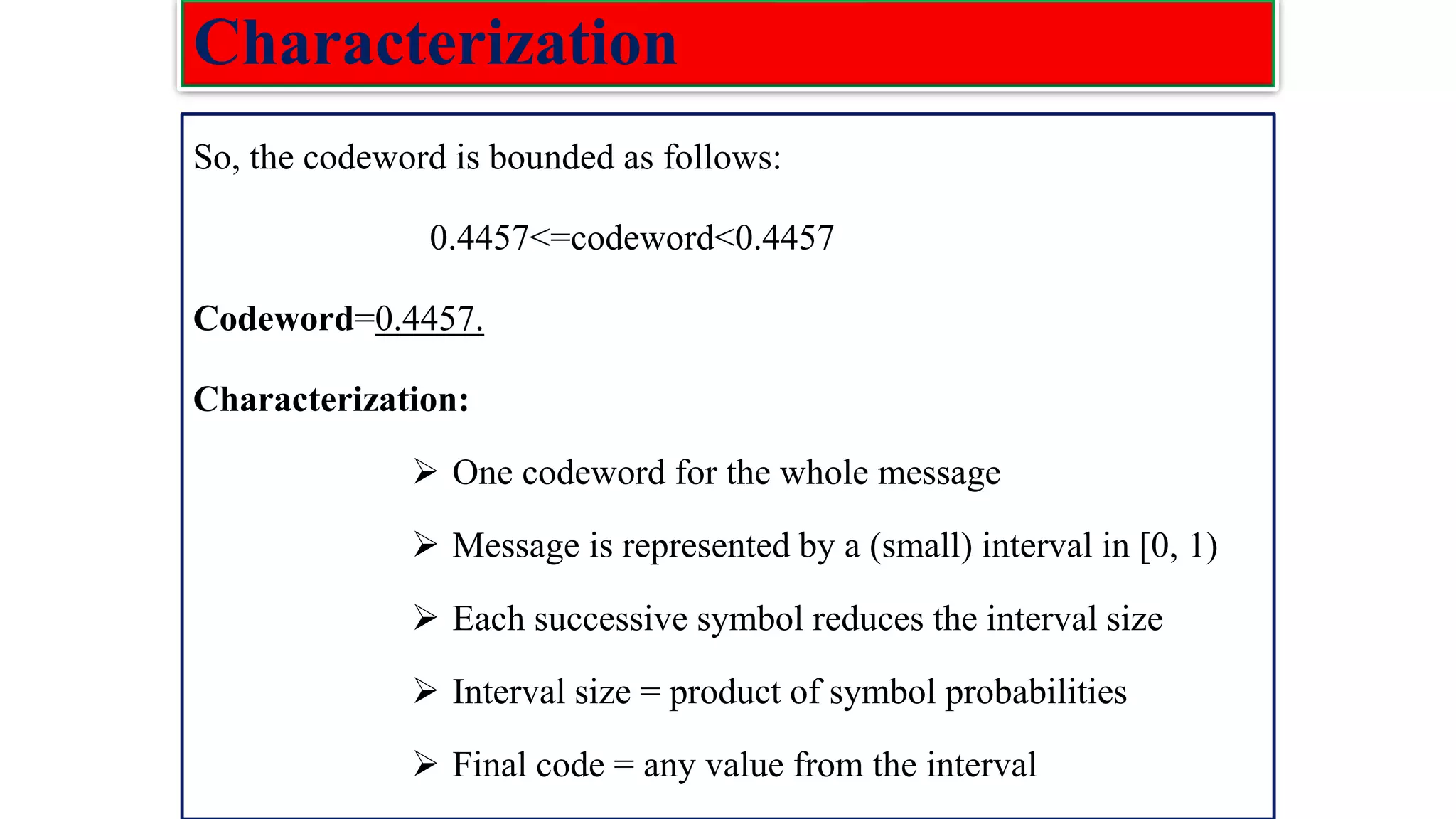
![algorithms 𝐼𝑅[𝐿,𝑅] = {[𝐿, 𝐿 + (𝑅 − 𝐿) 𝑞1),[L+(R-L) 𝑞1,L+(R-L) 𝑞2), [𝐿 + 𝑅 − 𝐿 𝑞2, 𝐿 + (𝑅 − 𝐿) 𝑞3),[L+(R-L) 𝑞𝑁−1,L+(R-L))} ❑ Using these definitions the arithmetic encoding is determined by the Following algorithm: ArithmeticEncoding ( Message ) 1. CurrentInterval = [0, 1); While the end of message is not reached 2. Read letter 𝒙𝒊 from the message; 3. Divid CurrentInterval into subintervals 𝑰𝑹𝑪𝒖𝒓𝒓𝒆𝒏𝒕𝑰𝒏𝒕𝒆𝒓𝒗𝒂𝒍; Output any number from the CurrentInterval (usually its left boundary);](https://image.slidesharecdn.com/coding-230511112653-d56c6b69/75/coding-pdf-5-2048.jpg)
![Low density parity check(LDPC) codes Examples :The parity check matrix for (n=20, 𝑤𝑐=3, 𝑤𝑟=4) code constructed by Gallager is given as: H= [𝐻1 𝐻2 𝐻3] 𝐻1 Rows of : 𝐻1=n/𝑤𝑟=20/4=5 Columns of: 𝐻1=n=20 𝐻2 Rows of H: m= n/𝑤𝑟(𝑤𝑐) =5*3=15 Columns of H: n=20 𝐻3](https://image.slidesharecdn.com/coding-230511112653-d56c6b69/75/coding-pdf-22-2048.jpg)
![Low density parity check(LDPC) codes LDPC Encoding 1.Preprocessing Method ❑ Derive a generator matrix G from the parity check matrix H for LDPC codes by means of Gaussian elimination in modulo-2 arithmetic. ❑ As such this method can be viewed as the preprocessing method. 1-by-n code vector c is first partitioned as: C=[b:m] where m is k by 1message vector, and b is the n−k by 1 parity vector correspondingly. ❑ The parity check matrix H is partitioned as: 𝐻𝑇 =[𝐻1;𝐻2]; where H1 is a square matrix of dimensions (n − k)×(n − k), and H2 is a rectangular matrix of dimensions k × (n − k).](https://image.slidesharecdn.com/coding-230511112653-d56c6b69/75/coding-pdf-26-2048.jpg)
![Low density parity check(LDPC) codes ❑ Imposing the constraint C𝐻𝑇=0. [b:m][𝐻1;𝐻2]=0 or equivalently b𝐻1+m𝐻2=0. ❑ The vectors m and b are related by: b=mp ,p=𝐻2𝐻1 −1 ❑ where 𝐻1 −1 is the inverse matrix of 𝐻1, which is naturally defined in modulo-2 arithmetic. ❑ Finally, the generator matrix of LDPC codes is defined by: G=[p:𝐼𝑘] = [𝐻2𝐻1 −1 :𝐼𝑘]](https://image.slidesharecdn.com/coding-230511112653-d56c6b69/75/coding-pdf-27-2048.jpg)
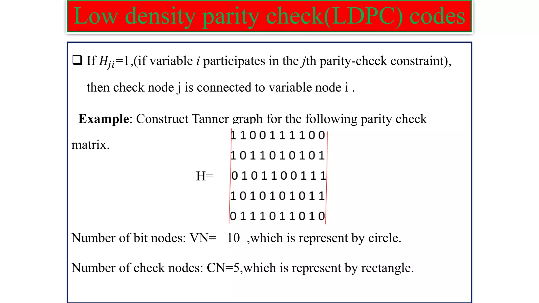
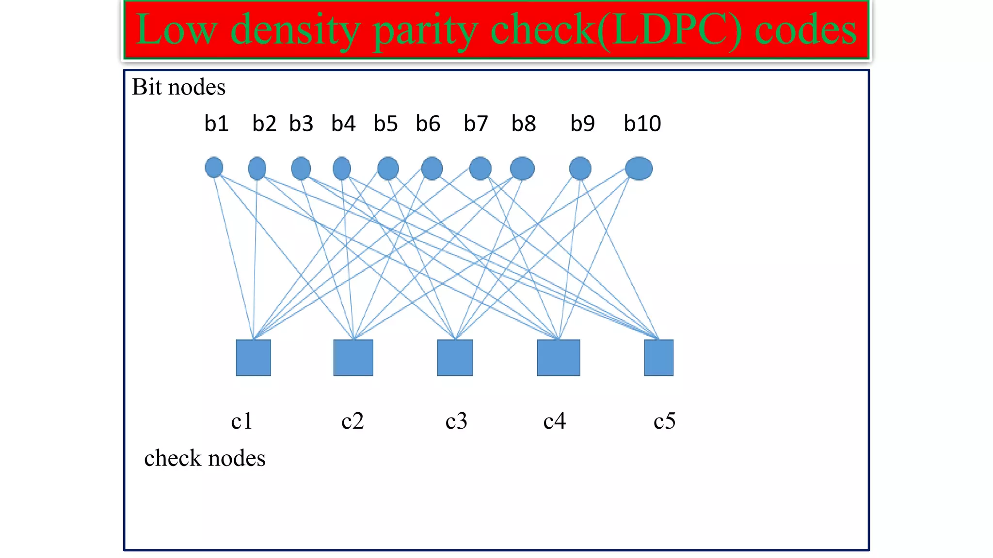
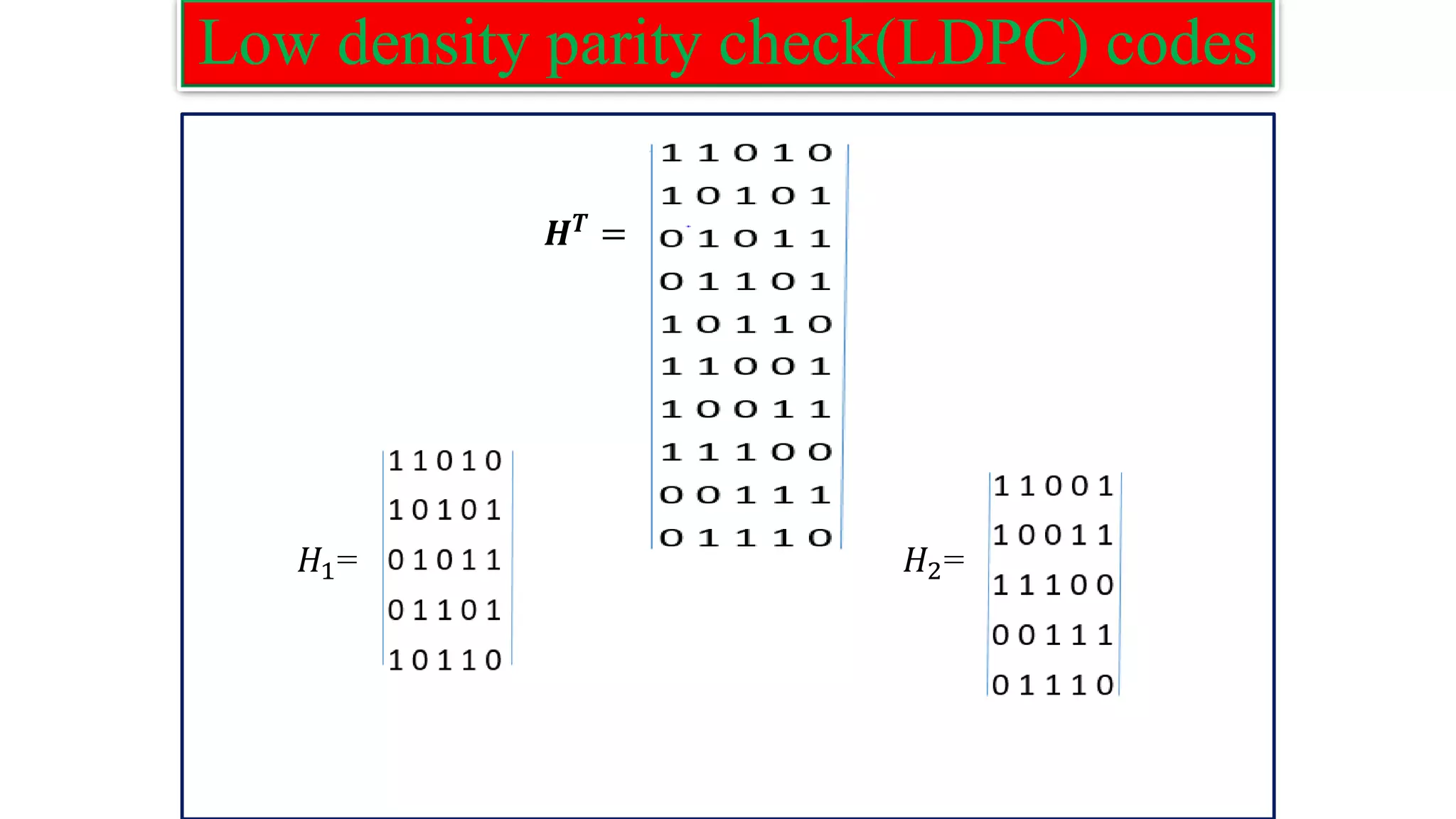
![Low density parity check(LDPC) codes ❑ The codeword can be generated as: C=mG Example: Construct LDPC code word for the following parity check matrix with the message vector m = [1 0 0 0 1]. H= Solution: The parity check matrix H is of the order 5 X 10 . ❑ We know that 𝑯𝑻 =[𝐻1;𝐻2]](https://image.slidesharecdn.com/coding-230511112653-d56c6b69/75/coding-pdf-28-2048.jpg)
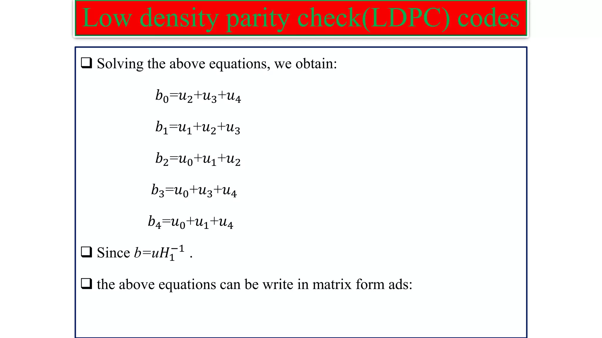
![Low density parity check(LDPC) codes ❑ Letting m𝐻1=u. [𝑏0 𝑏1 𝑏2 𝑏3 𝑏4] =[𝑢0 𝑢1 𝑢2 𝑢3 𝑢4] ❑ The above relation between b and u leads to the following equations: 𝑏0+𝑏1+𝑏4 = 𝑢𝑜 𝑏0+ 𝑏2+ 𝑏3 = 𝑢1 𝑏1+ 𝑏3+ 𝑏4 = 𝑢2 𝑏0+ 𝑏2+ 𝑏4 = 𝑢3 𝑏1+ 𝑏2+ 𝑏3 = 𝑢4](https://image.slidesharecdn.com/coding-230511112653-d56c6b69/75/coding-pdf-30-2048.jpg)
![Low density parity check(LDPC) codes b = [u] thus, 𝐻1 −1 = 𝐻2 𝐻1 −1 = =](https://image.slidesharecdn.com/coding-230511112653-d56c6b69/75/coding-pdf-32-2048.jpg)
![Low density parity check(LDPC) codes ❑ The generator matrix: G=[𝐻2 𝐻1 −1 𝐼𝑘]. G= ❑ The codeword can be generated as C=mG. C=[1 0 0 0 1] =[1 0 0 1 0 1 0 0 0 1].](https://image.slidesharecdn.com/coding-230511112653-d56c6b69/75/coding-pdf-33-2048.jpg)
![Low density parity check(LDPC) codes Step 3: Obtain 𝑝1 using the following: 𝐻𝐶𝑇=0,from this equation get 𝑝1. 𝑝1 𝑇 =−𝑑−1 (−𝐸𝑇−1 𝐴 + 𝐶)𝑠𝑇 Where d=−𝐸𝑇−1𝐵 + 𝐷 and s is message vector. Step 4: Obtain 𝑝2 using the following: 𝑝2 𝑇 =−𝑇−1(A𝑠𝑇+B𝑝1 𝑇 ) Step 5: Form the code vector c as: c = [s p1 p2] 𝑝1 holds the first g parity and 𝑝2 contains the remaining parity bits.](https://image.slidesharecdn.com/coding-230511112653-d56c6b69/75/coding-pdf-37-2048.jpg)