Classification (ML).ppt

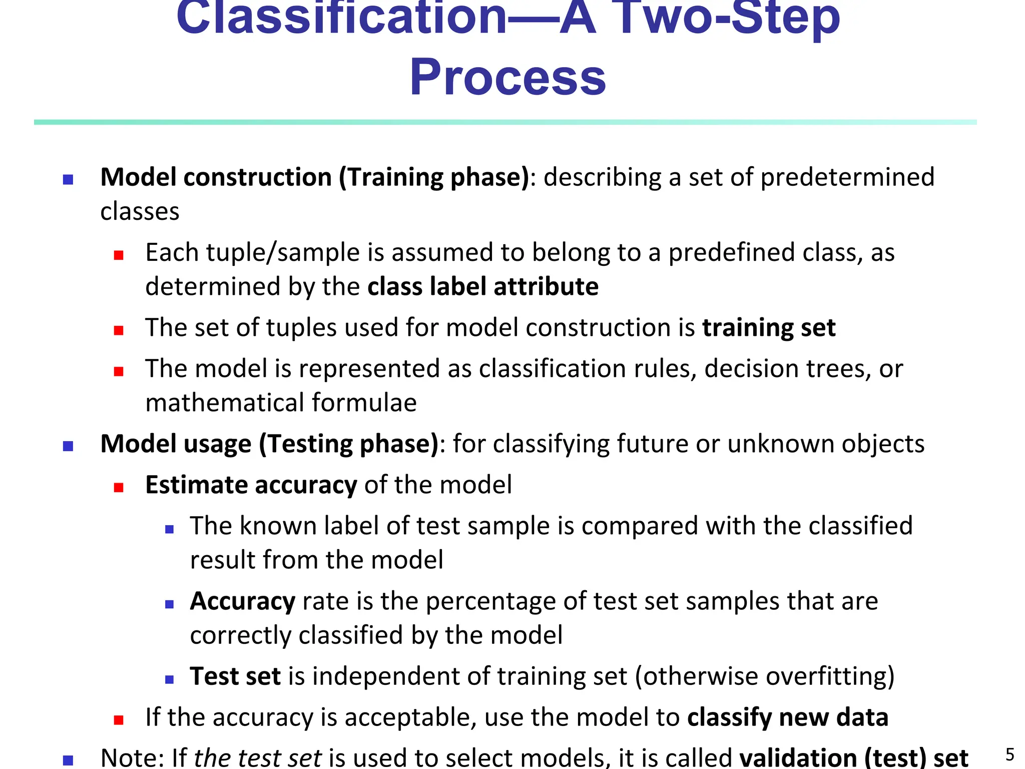
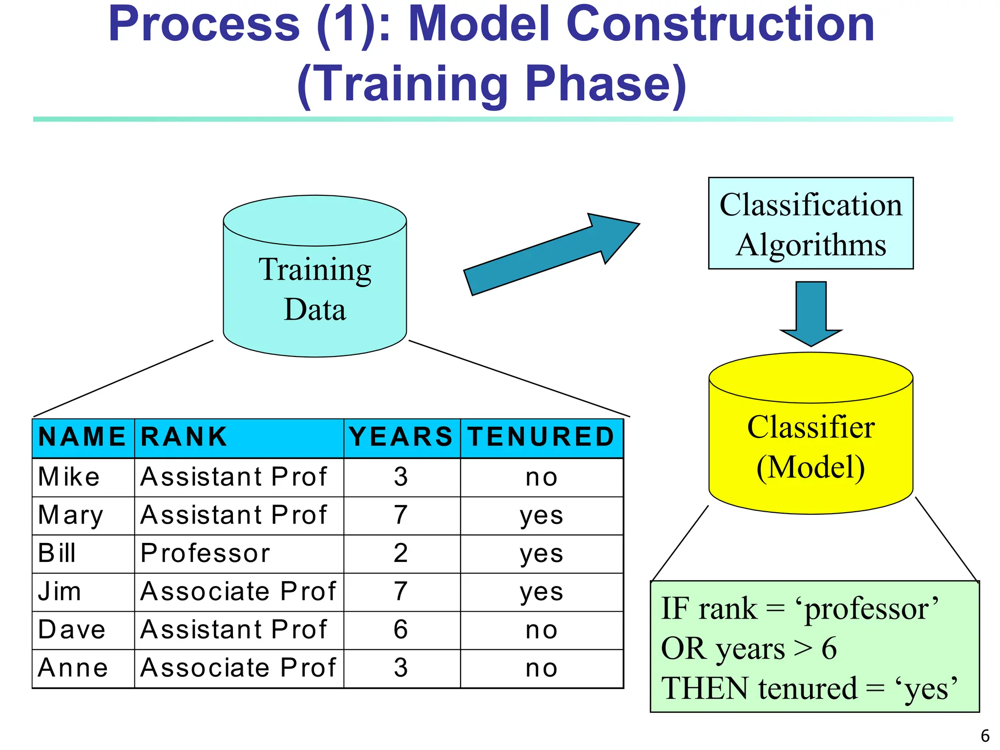
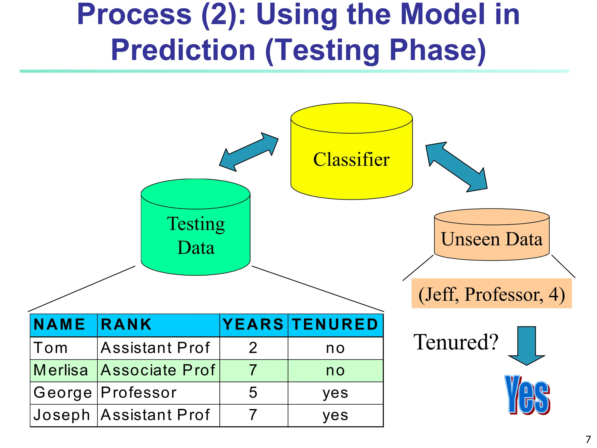
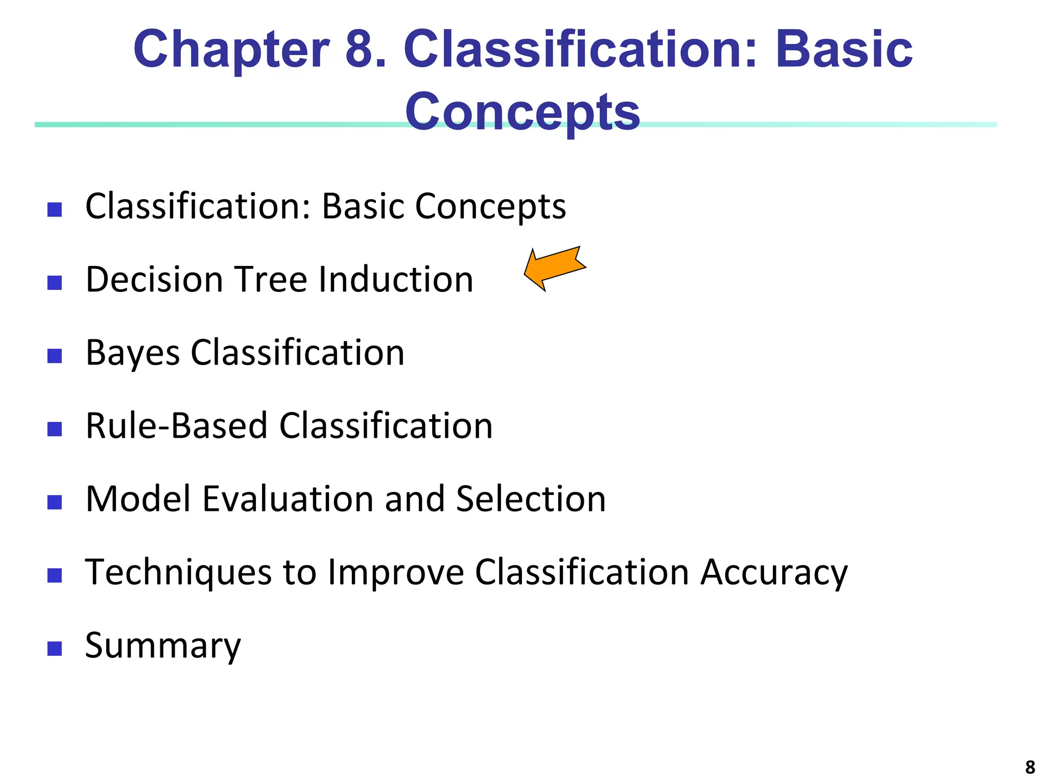
1 Machine Learning: Classification: Basic Concepts

2 Classification: Basic Concepts  Classification: Basic Concepts  Decision Tree Induction  Bayes Classification  Rule-Based Classification  Model Evaluation and Selection  Techniques to Improve Classification Accuracy  Summary

3 Supervised vs. Unsupervised Learning  Supervised learning (classification)  Supervision: The training data (observations, measurements, etc.) with labels indicating the class of the observations  New data is classified based on the training set

4  Classification  predicts categorical class labels (discrete or nominal)  classifies data (constructs a model) based on the training set and the values (class labels) in a classifying attribute and uses it in classifying new data  Numeric Prediction  models continuous-valued functions, i.e., predicts unknown or missing values  Typical applications  Credit/loan approval:  Medical diagnosis: if a tumor is cancerous or benign  Fraud detection: if a transaction is fraudulent  Web page categorization: which category it is Prediction Problems: Classification vs. Numeric Prediction

5 Classification—A Two-Step Process  Model construction (Training phase): describing a set of predetermined classes  Each tuple/sample is assumed to belong to a predefined class, as determined by the class label attribute  The set of tuples used for model construction is training set  The model is represented as classification rules, decision trees, or mathematical formulae  Model usage (Testing phase): for classifying future or unknown objects  Estimate accuracy of the model  The known label of test sample is compared with the classified result from the model  Accuracy rate is the percentage of test set samples that are correctly classified by the model  Test set is independent of training set (otherwise overfitting)  If the accuracy is acceptable, use the model to classify new data  Note: If the test set is used to select models, it is called validation (test) set

6 Process (1): Model Construction (Training Phase) Training Data NAME RANK YEARS TENURED Mike Assistant Prof 3 no Mary Assistant Prof 7 yes Bill Professor 2 yes Jim Associate Prof 7 yes Dave Assistant Prof 6 no Anne Associate Prof 3 no Classification Algorithms IF rank = ‘professor’ OR years > 6 THEN tenured = ‘yes’ Classifier (Model)

7 Process (2): Using the Model in Prediction (Testing Phase) Classifier Testing Data NAME RANK YEARS TENURED Tom Assistant Prof 2 no Merlisa Associate Prof 7 no George Professor 5 yes Joseph Assistant Prof 7 yes Unseen Data (Jeff, Professor, 4) Tenured?

8 Chapter 8. Classification: Basic Concepts  Classification: Basic Concepts  Decision Tree Induction  Bayes Classification  Rule-Based Classification  Model Evaluation and Selection  Techniques to Improve Classification Accuracy  Summary

9 Decision Tree Induction: An Example age? overcast student? credit rating? <=30 >40 no yes yes yes 31..40 fair excellent yes no age income student credit_rating buys_computer <=30 high no fair no <=30 high no excellent no 31…40 high no fair yes >40 medium no fair yes >40 low yes fair yes >40 low yes excellent no 31…40 low yes excellent yes <=30 medium no fair no <=30 low yes fair yes >40 medium yes fair yes <=30 medium yes excellent yes 31…40 medium no excellent yes 31…40 high yes fair yes >40 medium no excellent no  Training data set: Buys_computer  The data set follows an example of Quinlan’s ID3 (Playing Tennis)  Resulting tree:

10 Algorithm for Decision Tree Induction  Basic algorithm (a greedy algorithm)  Tree is constructed in a top-down recursive divide-and- conquer manner  At start, all the training examples are at the root  Attributes are categorical (if continuous-valued, they are discretized in advance)  Examples are partitioned recursively based on selected attributes  Test attributes are selected on the basis of a heuristic or statistical measure (e.g., information gain)  Conditions for stopping partitioning  All samples for a given node belong to the same class  There are no remaining attributes for further partitioning – majority voting is employed for classifying the leaf  There are no samples left

Brief Review of Entropy  11 m = 2

12 Attribute Selection Measure: Information Gain (ID3/C4.5)  Select the attribute with the highest information gain  Let pi be the probability that an arbitrary tuple in D belongs to class Ci, estimated by |Ci, D|/|D|  Expected information (entropy) needed to classify a tuple in D:  Information needed (after using A to split D into v partitions) to classify D:  Information gained by branching on attribute A ) ( log ) ( 2 1 i m i i p p D Info     ) ( | | | | ) ( 1 j v j j A D Info D D D Info     (D) Info Info(D) Gain(A) A  

13 Attribute Selection: Information Gain  Class Y: buys_computer = “yes”  Class N: buys_computer = “no” means “age <=30” has 5 out of 14 samples, with 2 yes’es and 3 no’s. Hence Similarly, age Y N I(Y, N) <=30 2 3 0.971 31…40 4 0 0 >40 3 2 0.971 694 . 0 ) 2 , 3 ( 14 5 ) 0 , 4 ( 14 4 ) 3 , 2 ( 14 5 ) (     I I I D Infoage 048 . 0 ) _ ( 151 . 0 ) ( 029 . 0 ) (    rating credit Gain student Gain income Gain 246 . 0 ) ( ) ( ) (    D Info D Info age Gain age age income student credit_rating buys_computer <=30 high no fair no <=30 high no excellent no 31…40 high no fair yes >40 medium no fair yes >40 low yes fair yes >40 low yes excellent no 31…40 low yes excellent yes <=30 medium no fair no <=30 low yes fair yes >40 medium yes fair yes <=30 medium yes excellent yes 31…40 medium no excellent yes 31…40 high yes fair yes >40 medium no excellent no ) 3 , 2 ( 14 5 I 940 . 0 ) 14 5 ( log 14 5 ) 14 9 ( log 14 9 ) 5 , 9 ( ) ( 2 2      I D Info

14 Comparing Attribute Selection Measures  The three measures, in general, return good results but  Information gain:  biased towards multivalued attributes  Gain ratio:  tends to prefer unbalanced splits in which one partition is much smaller than the others  Gini index:  biased to multivalued attributes  has difficulty when # of classes is large  tends to favor tests that result in equal-sized partitions and purity in both partitions

15 Gain Ratio for Attribute Selection (C4.5)  Information gain measure is biased towards attributes with a large number of values  C4.5 (a successor of ID3) uses gain ratio to overcome the problem (normalization to information gain)  GainRatio(A) = Gain(A)/SplitInfo(A)  Ex.  gain_ratio(income) = 0.029/1.557 = 0.019  The attribute with the maximum gain ratio is selected as the splitting attribute ) | | | | ( log | | | | ) ( 2 1 D D D D D SplitInfo j v j j A     

16 Computing Information-Gain for Continuous-Valued Attributes  Let attribute A be a continuous-valued attribute  Must determine the best split point for A  Sort the value A in increasing order  Typically, the midpoint between each pair of adjacent values is considered as a possible split point  (ai+ai+1)/2 is the midpoint between the values of ai and ai+1  The point with the minimum expected information requirement for A is selected as the split-point for A  Split:  D1 is the set of tuples in D satisfying A ≤ split-point, and D2 is the set of tuples in D satisfying A > split-point

17 Gini Index (CART, IBM IntelligentMiner)  If a data set D contains examples from n classes, gini index, gini(D) is defined as where pj is the relative frequency of class j in D  If a data set D is split on A into two subsets D1 and D2, then gini index gini(D) is defined as  Reduction in Impurity:  The attribute provides the smallest ginisplit(D) (or the largest reduction in impurity) is chosen to split the node (need to enumerate all the possible splitting points for each attribute)     n j p j D gini 1 2 1 ) ( ) ( | | | | ) ( | | | | ) ( 2 2 1 1 D gini D D D gini D D D giniA   ) ( ) ( ) ( D gini D gini A gini A   

18 Computation of Gini Index  Ex. D has 9 tuples in buys_computer = “yes” and 5 in “no”  Suppose the attribute income partitions D into 10 in D1: {low, medium} and 4 in D2 Gini{low,high} is 0.458; Gini{medium,high} is 0.450. Thus, split on the {low,medium} (and {high}) since it has the lowest Gini index  All attributes are assumed continuous-valued  May need other tools, e.g., clustering, to get the possible split values  Can be modified for categorical attributes 459 . 0 14 5 14 9 1 ) ( 2 2                 D gini ) ( 14 4 ) ( 14 10 ) ( 2 1 } , { D Gini D Gini D gini medium low income               

19 Other Attribute Selection Measures  CHAID: a popular decision tree algorithm, measure based on χ2 test for independence  C-SEP: performs better than info. gain and gini index in certain cases  G-statistic: has a close approximation to χ2 distribution  MDL (Minimal Description Length) principle (i.e., the simplest solution is preferred):  The best tree as the one that requires the fewest # of bits to both (1) encode the tree, and (2) encode the exceptions to the tree  Multivariate splits (partition based on multiple variable combinations)  CART: finds multivariate splits based on a linear comb. of attrs.  Which attribute selection measure is the best?  Most give good results, none is significantly superior than others

20 Overfitting and Tree Pruning  Overfitting: An induced tree may overfit the training data  Too many branches, some may reflect anomalies due to noise or outliers  Poor accuracy for unseen samples  Two approaches to avoid overfitting  Prepruning: Halt tree construction early ̵ do not split a node if this would result in the goodness measure falling below a threshold  Difficult to choose an appropriate threshold  Postpruning: Remove branches from a “fully grown” tree— get a sequence of progressively pruned trees  Use a set of data different from the training data to decide which is the “best pruned tree”

21 Enhancements to Basic Decision Tree Induction  Allow for continuous-valued attributes  Dynamically define new discrete-valued attributes that partition the continuous attribute value into a discrete set of intervals  Handle missing attribute values  Assign the most common value of the attribute  Assign probability to each of the possible values  Attribute construction  Create new attributes based on existing ones that are sparsely represented  This reduces fragmentation, repetition, and replication

22 Classification in Large Databases  Classification—a classical problem extensively studied by statisticians and machine learning researchers  Scalability: Classifying data sets with millions of examples and hundreds of attributes with reasonable speed  Why is decision tree induction popular?  relatively faster learning speed (than other classification methods)  convertible to simple and easy to understand classification rules  comparable classification accuracy with other methods

23 BOAT (Bootstrapped Optimistic Algorithm for Tree Construction)  Use a statistical technique called bootstrapping to create several smaller samples (subsets), each fits in memory  Each subset is used to create a tree, resulting in several trees  These trees are examined and used to construct a new tree T’  It turns out that T’ is very close to the tree that would be generated using the whole data set together

24 Classification: Basic Concepts  Classification: Basic Concepts  Decision Tree Induction  Bayes Classification Methods  Rule-Based Classification  Model Evaluation and Selection  Techniques to Improve Classification Accuracy: Ensemble Methods  Summary

25 Bayesian Classification: Why?  A statistical classifier: performs probabilistic prediction, i.e., predicts class membership probabilities  Foundation: Based on Bayes’ Theorem.  Performance: A simple Bayesian classifier, naïve Bayesian classifier, has comparable performance with decision tree and selected neural network classifiers  Incremental: Each training example can incrementally increase/decrease the probability that a hypothesis is correct — prior knowledge can be combined with observed data  Standard: Even when Bayesian methods are computationally intractable, they can provide a standard of optimal decision making against which other methods can be measured

26 Bayes’ Theorem: Basics  Total probability Theorem:  Bayes’ Theorem:  Let X be a data sample (“evidence”): class label is unknown  Let H be a hypothesis that X belongs to class C  Classification is to determine P(H|X), (i.e., posteriori probability): the probability that the hypothesis holds given the observed data sample X  P(H) (prior probability): the initial probability  E.g., X will buy computer, regardless of age, income, …  P(X): probability that sample data is observed  P(X|H) (likelihood): the probability of observing the sample X, given that the hypothesis holds  E.g., Given that X will buy computer, the prob. that X is 31..40, medium income ) ( ) 1 | ( ) ( i A P M i i A B P B P    ) ( / ) ( ) | ( ) ( ) ( ) | ( ) | ( X X X X X P H P H P P H P H P H P   

27 Prediction Based on Bayes’ Theorem  Given training data X, posteriori probability of a hypothesis H, P(H|X), follows the Bayes’ theorem  Informally, this can be viewed as posteriori = likelihood x prior/evidence  Predicts X belongs to Ci iff the probability P(Ci|X) is the highest among all the P(Ck|X) for all the k classes  Practical difficulty: It requires initial knowledge of many probabilities, involving significant computational cost ) ( / ) ( ) | ( ) ( ) ( ) | ( ) | ( X X X X X P H P H P P H P H P H P   

28 Classification Is to Derive the Maximum Posteriori  Let D be a training set of tuples and their associated class labels, and each tuple is represented by an n-D attribute vector X = (x1, x2, …, xn)  Suppose there are m classes C1, C2, …, Cm.  Classification is to derive the maximum posteriori, i.e., the maximal P(Ci|X)  This can be derived from Bayes’ theorem  Since P(X) is constant for all classes, only needs to be maximized ) ( ) ( ) | ( ) | ( X X X P i C P i C P i C P  ) ( ) | ( ) | ( i C P i C P i C P X X 

29 Naïve Bayes Classifier  A simplified assumption: attributes are conditionally independent (i.e., no dependence relation between attributes):  This greatly reduces the computation cost: Only counts the class distribution  If Ak is categorical, P(xk|Ci) is the # of tuples in Ci having value xk for Ak divided by |Ci, D| (# of tuples of Ci in D)  If Ak is continous-valued, P(xk|Ci) is usually computed based on Gaussian distribution with a mean μ and standard deviation σ and P(xk|Ci) is ) | ( ... ) | ( ) | ( 1 ) | ( ) | ( 2 1 Ci x P Ci x P Ci x P n k Ci x P Ci P n k        X 2 2 2 ) ( 2 1 ) , , (          x e x g ) , , ( ) | ( i i C C k x g Ci P    X

30 Naïve Bayes Classifier: Training Dataset Class: C1:buys_computer = ‘yes’ C2:buys_computer = ‘no’ Data to be classified: X = (age <=30, Income = medium, Student = yes Credit_rating = Fair) age income student credit_rating buys_compu <=30 high no fair no <=30 high no excellent no 31…40 high no fair yes >40 medium no fair yes >40 low yes fair yes >40 low yes excellent no 31…40 low yes excellent yes <=30 medium no fair no <=30 low yes fair yes >40 medium yes fair yes <=30 medium yes excellent yes 31…40 medium no excellent yes 31…40 high yes fair yes >40 medium no excellent no

31 Naïve Bayes Classifier: An Example  P(Ci): P(buys_computer = “yes”) = 9/14 = 0.643 P(buys_computer = “no”) = 5/14= 0.357  Compute P(X|Ci) for each class P(age = “<=30” | buys_computer = “yes”) = 2/9 = 0.222 P(age = “<= 30” | buys_computer = “no”) = 3/5 = 0.6 P(income = “medium” | buys_computer = “yes”) = 4/9 = 0.444 P(income = “medium” | buys_computer = “no”) = 2/5 = 0.4 P(student = “yes” | buys_computer = “yes) = 6/9 = 0.667 P(student = “yes” | buys_computer = “no”) = 1/5 = 0.2 P(credit_rating = “fair” | buys_computer = “yes”) = 6/9 = 0.667 P(credit_rating = “fair” | buys_computer = “no”) = 2/5 = 0.4  X = (age <= 30 , income = medium, student = yes, credit_rating = fair) P(X|Ci) : P(X|buys_computer = “yes”) = 0.222 x 0.444 x 0.667 x 0.667 = 0.044 P(X|buys_computer = “no”) = 0.6 x 0.4 x 0.2 x 0.4 = 0.019 P(X|Ci)*P(Ci) : P(X|buys_computer = “yes”) * P(buys_computer = “yes”) = 0.028 P(X|buys_computer = “no”) * P(buys_computer = “no”) = 0.007 Therefore, X belongs to class (“buys_computer = yes”) age income student credit_rating buys_comp <=30 high no fair no <=30 high no excellent no 31…40 high no fair yes >40 medium no fair yes >40 low yes fair yes >40 low yes excellent no 31…40 low yes excellent yes <=30 medium no fair no <=30 low yes fair yes >40 medium yes fair yes <=30 medium yes excellent yes 31…40 medium no excellent yes 31…40 high yes fair yes >40 medium no excellent no

32 Avoiding the Zero-Probability Problem  Naïve Bayesian prediction requires each conditional prob. be non-zero. Otherwise, the predicted prob. will be zero  Ex. Suppose a dataset with 1000 tuples, income=low (0), income= medium (990), and income = high (10)  Use Laplacian correction (or Laplacian estimator)  Adding 1 to each case Prob(income = low) = 1/1003 Prob(income = medium) = 991/1003 Prob(income = high) = 11/1003  The “corrected” prob. estimates are close to their “uncorrected” counterparts    n k Ci xk P Ci X P 1 ) | ( ) | (

33 Naïve Bayes Classifier: Comments  Advantages  Easy to implement  Good results obtained in most of the cases  Disadvantages  Assumption: class conditional independence, therefore loss of accuracy  Practically, dependencies exist among variables  E.g., hospitals: patients: Profile: age, family history, etc. Symptoms: fever, cough etc., Disease: lung cancer, diabetes, etc.  Dependencies among these cannot be modeled by Naïve Bayes Classifier  How to deal with these dependencies? Bayesian Belief Networks (Chapter 9)

34 Chapter 8. Classification: Basic Concepts  Classification: Basic Concepts  Decision Tree Induction  Bayes Classification Methods  Rule-Based Classification  Model Evaluation and Selection  Techniques to Improve Classification Accuracy: Ensemble Methods  Summary

35 Using IF-THEN Rules for Classification  Represent the knowledge in the form of IF-THEN rules R: IF age = youth AND student = yes THEN buys_computer = yes  Rule antecedent/precondition vs. rule consequent  Assessment of a rule: coverage and accuracy  ncovers = # of tuples covered by R  ncorrect = # of tuples correctly classified by R coverage(R) = ncovers /|D| /* D: training data set */ accuracy(R) = ncorrect / ncovers  If more than one rule are triggered, need conflict resolution  Size ordering: assign the highest priority to the triggering rules that has the “toughest” requirement (i.e., with the most attribute tests)  Class-based ordering: decreasing order of prevalence or misclassification cost per class  Rule-based ordering (decision list): rules are organized into one long priority list, according to some measure of rule quality or by experts

36 age? student? credit rating? <=30 >40 no yes yes yes 31..40 fair excellent yes no  Example: Rule extraction from our buys_computer decision-tree IF age = young AND student = no THEN buys_computer = no IF age = young AND student = yes THEN buys_computer = yes IF age = mid-age THEN buys_computer = yes IF age = old AND credit_rating = excellent THEN buys_computer = no IF age = old AND credit_rating = fair THEN buys_computer = yes Rule Extraction from a Decision Tree  Rules are easier to understand than large trees  One rule is created for each path from the root to a leaf  Each attribute-value pair along a path forms a conjunction: the leaf holds the class prediction  Rules are mutually exclusive and exhaustive

37 Rule Induction: Sequential Covering Method  Sequential covering algorithm: Extracts rules directly from training data  Typical sequential covering algorithms: FOIL, AQ, CN2, RIPPER  Rules are learned sequentially, each for a given class Ci will cover many tuples of Ci but none (or few) of the tuples of other classes  Steps:  Rules are learned one at a time  Each time a rule is learned, the tuples covered by the rules are removed  Repeat the process on the remaining tuples until termination condition, e.g., when no more training examples or when the quality of a rule returned is below a user-specified threshold  Comp. w. decision-tree induction: learning a set of rules simultaneously

38 Sequential Covering Algorithm while (enough target tuples left) generate a rule remove positive target tuples satisfying this rule Examples covered by Rule 3 Examples covered by Rule 2 Examples covered by Rule 1 Positive examples

39 Rule Generation  To generate a rule while(true) find the best predicate p if foil-gain(p) > threshold then add p to current rule else break Positive examples Negative examples A3=1 A3=1&&A1=2 A3=1&&A1=2 &&A8=5

40 How to Learn-One-Rule?  Start with the most general rule possible: condition = empty  Adding new attributes by adopting a greedy depth-first strategy  Picks the one that most improves the rule quality  Rule-Quality measures: consider both coverage and accuracy  Rule Accuracy  Foil-gain (in FOIL & RIPPER): assesses info_gain by extending condition ) log ' ' ' (log ' _ 2 2 neg pos pos neg pos pos pos Gain FOIL     

Model Evaluation and Selection  Evaluation metrics: How can we measure accuracy? Other metrics to consider?  Use validation test set of class-labeled tuples instead of training set when assessing accuracy  Methods for estimating a classifier’s accuracy:  Holdout method, random subsampling  Cross-validation  Bootstrap  Comparing classifiers:  Confidence intervals  Cost-benefit analysis and ROC Curves 42

Classifier Evaluation Metrics: Confusion Matrix Actual classPredicted class buy_computer = yes buy_computer = no Total buy_computer = yes 6954 46 7000 buy_computer = no 412 2588 3000 Total 7366 2634 10000  Given m classes, an entry, CMi,j in a confusion matrix indicates # of tuples in class i that were labeled by the classifier as class j  May have extra rows/columns to provide totals Confusion Matrix: Actual classPredicted class C1 ¬ C1 C1 True Positives (TP) False Negatives (FN) ¬ C1 False Positives (FP) True Negatives (TN) Example of Confusion Matrix: 43

Accuracy, Error Rate, Sensitivity and Specificity  Classifier Accuracy, or recognition rate: percentage of test set tuples that are correctly classified Accuracy = (TP + TN)/All  Error rate: 1 – accuracy, or Error rate = (FP + FN)/All  Class Imbalance Problem:  One class may be rare, e.g. fraud, or HIV-positive  Significant majority of the negative class and minority of the positive class  Sensitivity: True Positive recognition rate  Sensitivity = TP/P  Specificity: True Negative recognition rate  Specificity = TN/N AP C ¬C C TP FN P ¬C FP TN N P’ N’ All 44

Precision and Recall, and F- measures  Precision: exactness – what % of tuples that the classifier labeled as positive are actually positive  Recall: completeness – what % of positive tuples did the classifier label as positive?  Perfect score is 1.0  Inverse relationship between precision & recall  F measure (F1 or F-score): harmonic mean of precision and recall,  Fß: weighted measure of precision and recall  assigns ß times as much weight to recall as to precision 45

Classifier Evaluation Metrics: Example 46  Precision = 90/230 = 39.13% Recall = 90/300 = 30.00% Actual ClassPredicted class cancer = yes cancer = no Total Recognition(%) cancer = yes 90 210 300 30.00 (sensitivity cancer = no 140 9560 9700 98.56 (specificity) Total 230 9770 10000 96.40 (accuracy)

Holdout & Cross-Validation Methods  Holdout method  Given data is randomly partitioned into two independent sets  Training set (e.g., 2/3) for model construction  Test set (e.g., 1/3) for accuracy estimation  Random sampling: a variation of holdout  Repeat holdout k times, accuracy = avg. of the accuracies obtained  Cross-validation (k-fold, where k = 10 is most popular)  Randomly partition the data into k mutually exclusive subsets, each approximately equal size  At i-th iteration, use Di as test set and others as training set  Leave-one-out: k folds where k = # of tuples, for small sized data  *Stratified cross-validation*: folds are stratified so that class dist. in each fold is approx. the same as that in the initial data 47

Evaluating Classifier Accuracy: Bootstrap  Bootstrap  Works well with small data sets  Samples the given training tuples uniformly with replacement  i.e., each time a tuple is selected, it is equally likely to be selected again and re-added to the training set  Several bootstrap methods, and a common one is .632 boostrap  A data set with d tuples is sampled d times, with replacement, resulting in a training set of d samples. The data tuples that did not make it into the training set end up forming the test set. About 63.2% of the original data end up in the bootstrap, and the remaining 36.8% form the test set (since (1 – 1/d)d ≈ e-1 = 0.368)  Repeat the sampling procedure k times, overall accuracy of the model: 48

Estimating Confidence Intervals: Null Hypothesis  Friedman Test  Perform 10-fold cross-validation  Assume samples follow a normal distribution with k–1 degrees of freedom (here, k=10)  Use Friedman Test  Null Hypothesis (H0): M1 & M2 are the same and changes are merely random  If we can reject null hypothesis, then  we conclude that the difference between M1 & M2 is statistically significant 49

Estimating Confidence Intervals: Null Hypothesis Friedman Test  Find rank of classifier on datasets ( is the rank of the jth of k number of models on ith )  Find average rank  Find here N – No. of dataset, k – no. of classification model  Find FF statistic  Find crucial value (cv) from FF statistic with (k-1) and (k-1)*(N- 1) degree of freedom (Table of normal disribution) 50

Estimating Confidence Intervals: Null Hypothesis  If cv< FF statistic then Null-Hypothesis is rejected else Accepted  Example 51 Datasets Fitness Obtained by Various Hybrid Models A B C D F1 2.462398 (3) 2.462398 (3) 2.534043 (2) 3.057658 (1) F2 5.972679 (3) 5.97268 (2) 5.97268 (2) 9.411738 (1) F3 1.888252 (3) 1.869618 (4) 1.895258 (2) 3.118014 (1) F4 2.024735 (4) 2.033361 (3) 2.037116 (2) 3.057657 (1) F5 1.677268 (4) 1.696773 (2) 1.67727 (3) 2.382388 (1) F6 2.58331 (3) 2.813839 (2) 3.276094 (1) 2.349537 (4) F7 2.216361 (4) 2.216474 (3) 2.217241 (2) 2.220777 (1) F8 1.888252 (3) 1.869618 (4) 2.675806 (2) 3.118014 (1) F9 1.54692 (4) 1.547116 (3) 1.548419 (2) 2.162731 (1) F10 1.888967 (4) 1.981951 (3) 2.267907 (2) 3.690652 (1) F11 2.128121 (3) 2.127284 (4) 2.128124 (2) 2.696475 (1) Friedman’s Rank in Average 3.455 3 2 1.272

Estimating Confidence Intervals: Null Hypothesis 52

Model Selection: ROC Curves  ROC (Receiver Operating Characteristics) curves: for visual comparison of classification models  Originated from signal detection theory  Shows the trade-off between the true positive rate and the false positive rate  The area under the ROC curve is a measure of the accuracy of the model  Rank the test tuples in decreasing order: the one that is most likely to belong to the positive class appears at the top of the list  The closer to the diagonal line (i.e., the closer the area is to 0.5), the less accurate is the model  Vertical axis represents the true positive rate  Horizontal axis rep. the false positive rate  The plot also shows a diagonal line  A model with perfect accuracy will have an area of 1.0 53

Issues Affecting Model Selection  Accuracy  classifier accuracy: predicting class label  Speed  time to construct the model (training time)  time to use the model (classification/prediction time)  Robustness: handling noise and missing values  Scalability: efficiency in disk-resident databases  Interpretability  understanding and insight provided by the model  Other measures, e.g., goodness of rules, such as decision tree size or compactness of classification rules 54

Ensemble Methods: Increasing the Accuracy  Ensemble methods  Use a combination of models to increase accuracy  Combine a series of k learned models, M1, M2, …, Mk, with the aim of creating an improved model M*  Popular ensemble methods  Bagging: averaging the prediction over a collection of classifiers  Boosting: weighted vote with a collection of classifiers  Ensemble: combining a set of heterogeneous classifiers 56

Bagging: Boostrap Aggregation  Analogy: Diagnosis based on multiple doctors’ majority vote  Training  Given a set D of d tuples, at each iteration i, a training set Di of d tuples is sampled with replacement from D (i.e., bootstrap)  A classifier model Mi is learned for each training set Di  Classification: classify an unknown sample X  Each classifier Mi returns its class prediction  The bagged classifier M* counts the votes and assigns the class with the most votes to X  Prediction: can be applied to the prediction of continuous values by taking the average value of each prediction for a given test tuple  Accuracy  Often significantly better than a single classifier derived from D  For noise data: not considerably worse, more robust  Proved improved accuracy in prediction 57

Boosting  Analogy: Consult several doctors, based on a combination of weighted diagnoses—weight assigned based on the previous diagnosis accuracy  How boosting works?  Weights are assigned to each training tuple  A series of k classifiers is iteratively learned  After a classifier Mi is learned, the weights are updated to allow the subsequent classifier, Mi+1, to pay more attention to the training tuples that were misclassified by Mi  The final M* combines the votes of each individual classifier, where the weight of each classifier's vote is a function of its accuracy  Boosting algorithm can be extended for numeric prediction  Comparing with bagging: Boosting tends to have greater accuracy, but it also risks overfitting the model to misclassified data 58

59 Adaboost (Freund and Schapire, 1997)  Given a set of d class-labeled tuples, (X1, y1), …, (Xd, yd)  Initially, all the weights of tuples are set the same (1/d)  Generate k classifiers in k rounds. At round i,  Tuples from D are sampled (with replacement) to form a training set Di of the same size  Each tuple’s chance of being selected is based on its weight  A classification model Mi is derived from Di  Its error rate is calculated using Di as a test set  If a tuple is misclassified, its weight is increased, o.w. it is decreased  Error rate: err(Xj) is the misclassification error of tuple Xj. Classifier Mi error rate is the sum of the weights of the misclassified tuples:  The weight of classifier Mi’s vote is ) ( ) ( 1 log i i M error M error     d j j i err w M error ) ( ) ( j X

Random Forest (Breiman 2001)  Random Forest:  Each classifier in the ensemble is a decision tree classifier and is generated using a random selection of attributes at each node to determine the split  During classification, each tree votes and the most popular class is returned  Two Methods to construct Random Forest:  Forest-RI (random input selection): Randomly select, at each node, F attributes as candidates for the split at the node. The CART methodology is used to grow the trees to maximum size  Forest-RC (random linear combinations): Creates new attributes (or features) that are a linear combination of the existing attributes (reduces the correlation between individual classifiers)  Comparable in accuracy to Adaboost, but more robust to errors and outliers  Insensitive to the number of attributes selected for consideration at each split, and faster than bagging or boosting 60

Classification of Class-Imbalanced Data Sets  Class-imbalance problem: Rare positive example but numerous negative ones, e.g., medical diagnosis, fraud, oil-spill, fault, etc.  Traditional methods assume a balanced distribution of classes and equal error costs: not suitable for class-imbalanced data  Typical methods for imbalance data in 2-class classification:  Oversampling: re-sampling of data from positive class  Under-sampling: randomly eliminate tuples from negative class  Threshold-moving: moves the decision threshold, t, so that the rare class tuples are easier to classify, and hence, less chance of costly false negative errors  Ensemble techniques: Ensemble multiple classifiers introduced above  Still difficult for class imbalance problem on multiclass tasks 61

Classification (ML).ppt

More Related Content

What's hot

Similar to Classification (ML).ppt

Recently uploaded

In this document

Classification (ML).ppt