artificial-neural-networks overviewrev.ppt

Artificial Neural Networks : An Introduction G.Anuradha

Learning Objectives • Fundamentals of ANN • Comparison between biological neuron and artificial neuron • Basic models of ANN • Different types of connections of NN, Learning and activation function • Basic fundamental neuron model- McCulloch-Pitts neuron and Hebb network

Fundamental concept • NN are constructed and implemented to model the human brain. • Performs various tasks such as pattern- matching, classification, optimization function, approximation, vector quantization and data clustering. • These tasks are difficult for traditional computers

ANN • ANN posess a large number of processing elements called nodes/neurons which operate in parallel. • Neurons are connected with others by connection link. • Each link is associated with weights which contain information about the input signal. • Each neuron has an internal state of its own which is a function of the inputs that neuron receives- Activation level

Artificial Neural Networks x1 x2 X1 X2 w1 w2 Y y n X 1 1 2 2 in y x w x w   ( ) in y f y 

Neural net of pure linear eqn. Y X Input m mx

Information flow in nervous system

Neuron and a sample of pulse train

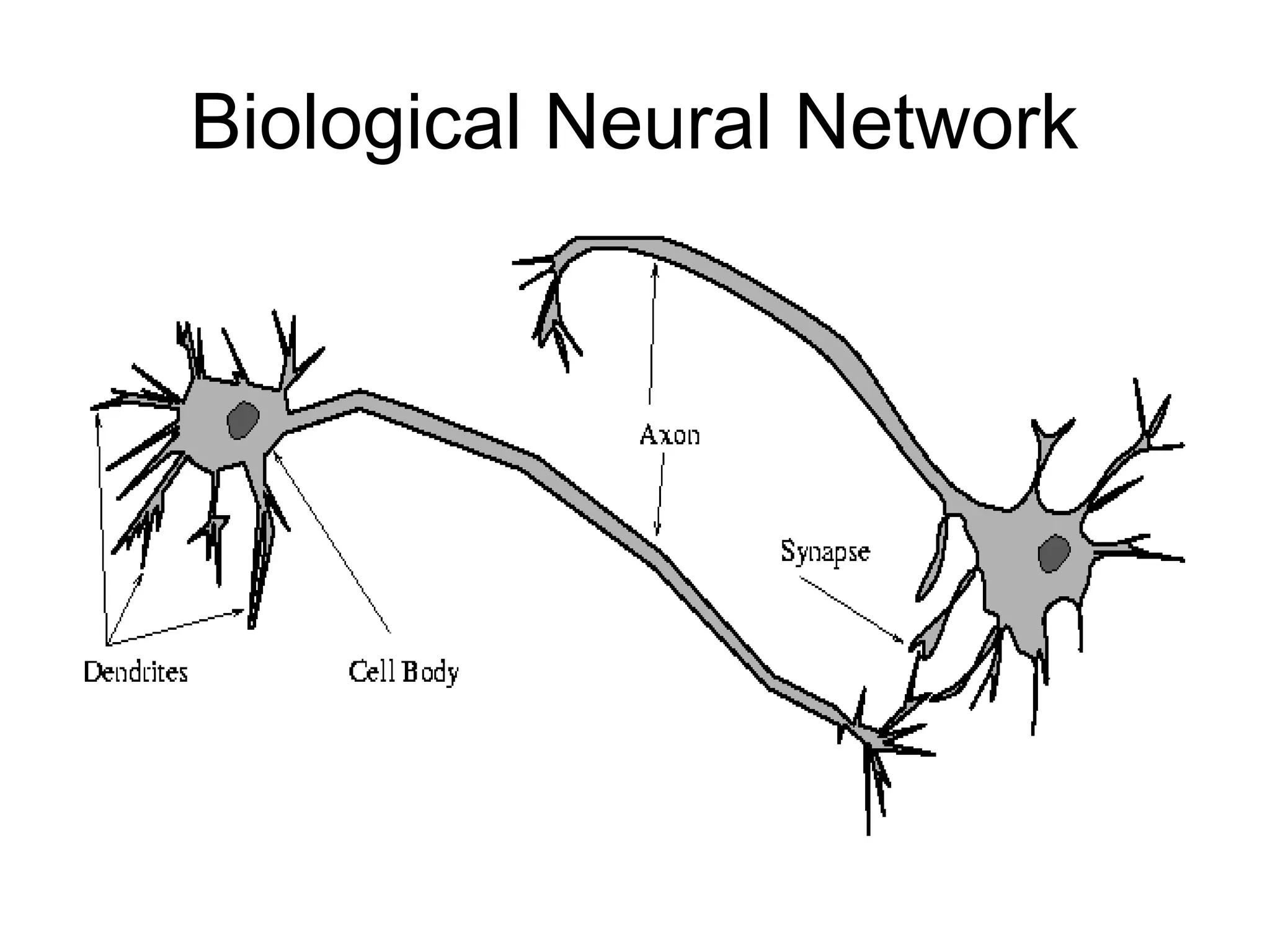
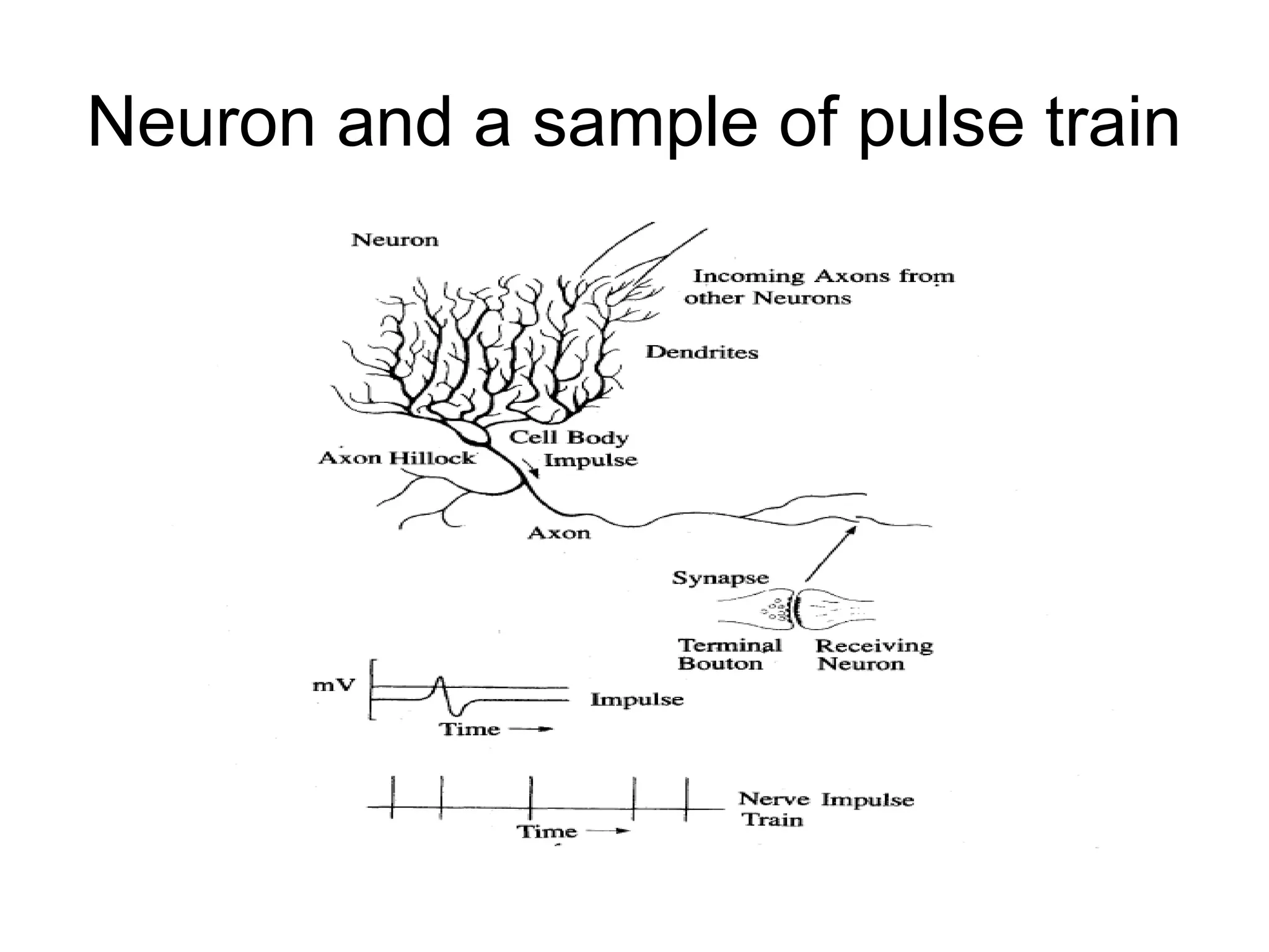
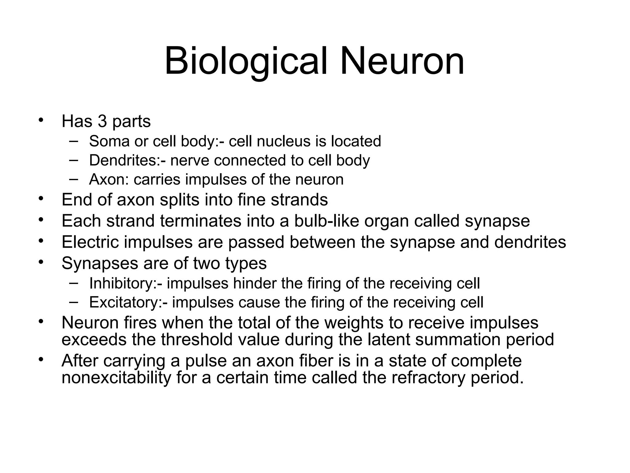
Biological Neuron • Has 3 parts – Soma or cell body:- cell nucleus is located – Dendrites:- nerve connected to cell body – Axon: carries impulses of the neuron • End of axon splits into fine strands • Each strand terminates into a bulb-like organ called synapse • Electric impulses are passed between the synapse and dendrites • Synapses are of two types – Inhibitory:- impulses hinder the firing of the receiving cell – Excitatory:- impulses cause the firing of the receiving cell • Neuron fires when the total of the weights to receive impulses exceeds the threshold value during the latent summation period • After carrying a pulse an axon fiber is in a state of complete nonexcitability for a certain time called the refractory period.

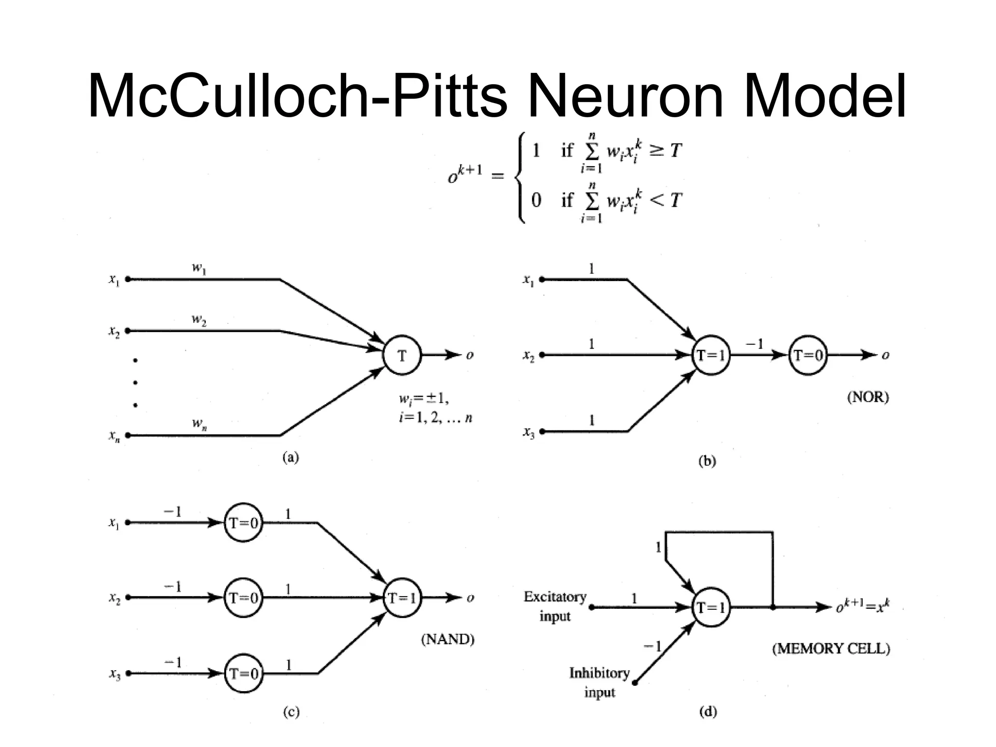
Features of McCulloch-Pitts model • Allows binary 0,1 states only • Operates under a discrete-time assumption • Weights and the neurons’ thresholds are fixed in the model and no interaction among network neurons • Just a primitive model

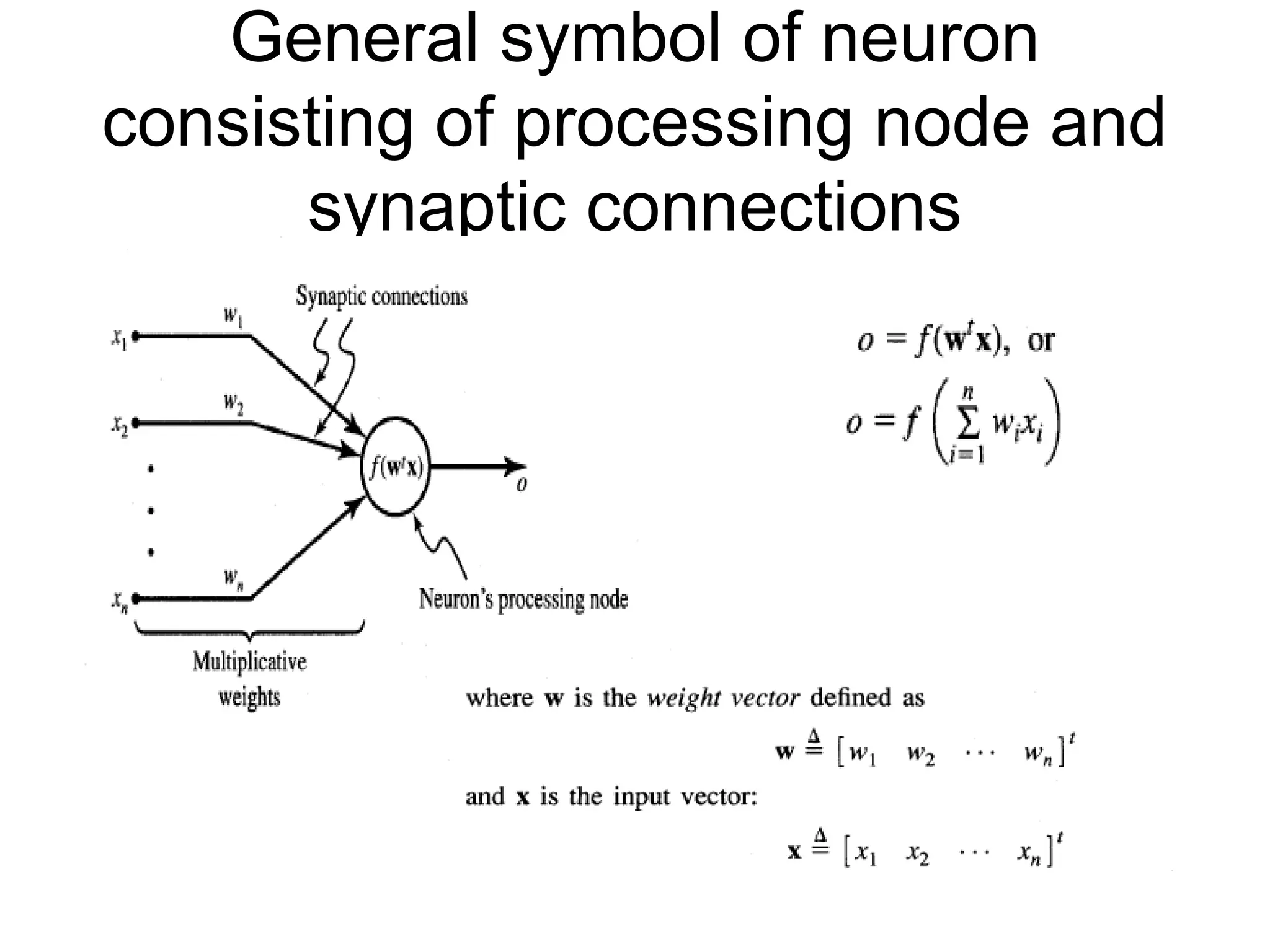
General symbol of neuron consisting of processing node and synaptic connections

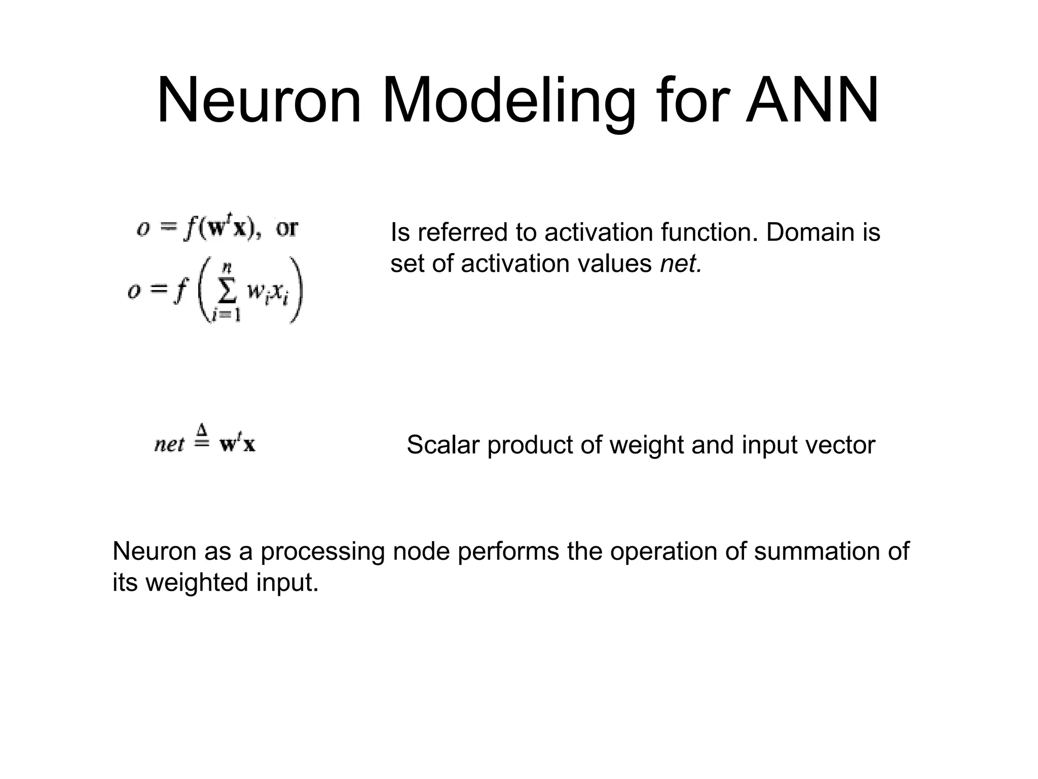
Neuron Modeling for ANN Is referred to activation function. Domain is set of activation values net. Scalar product of weight and input vector Neuron as a processing node performs the operation of summation of its weighted input.

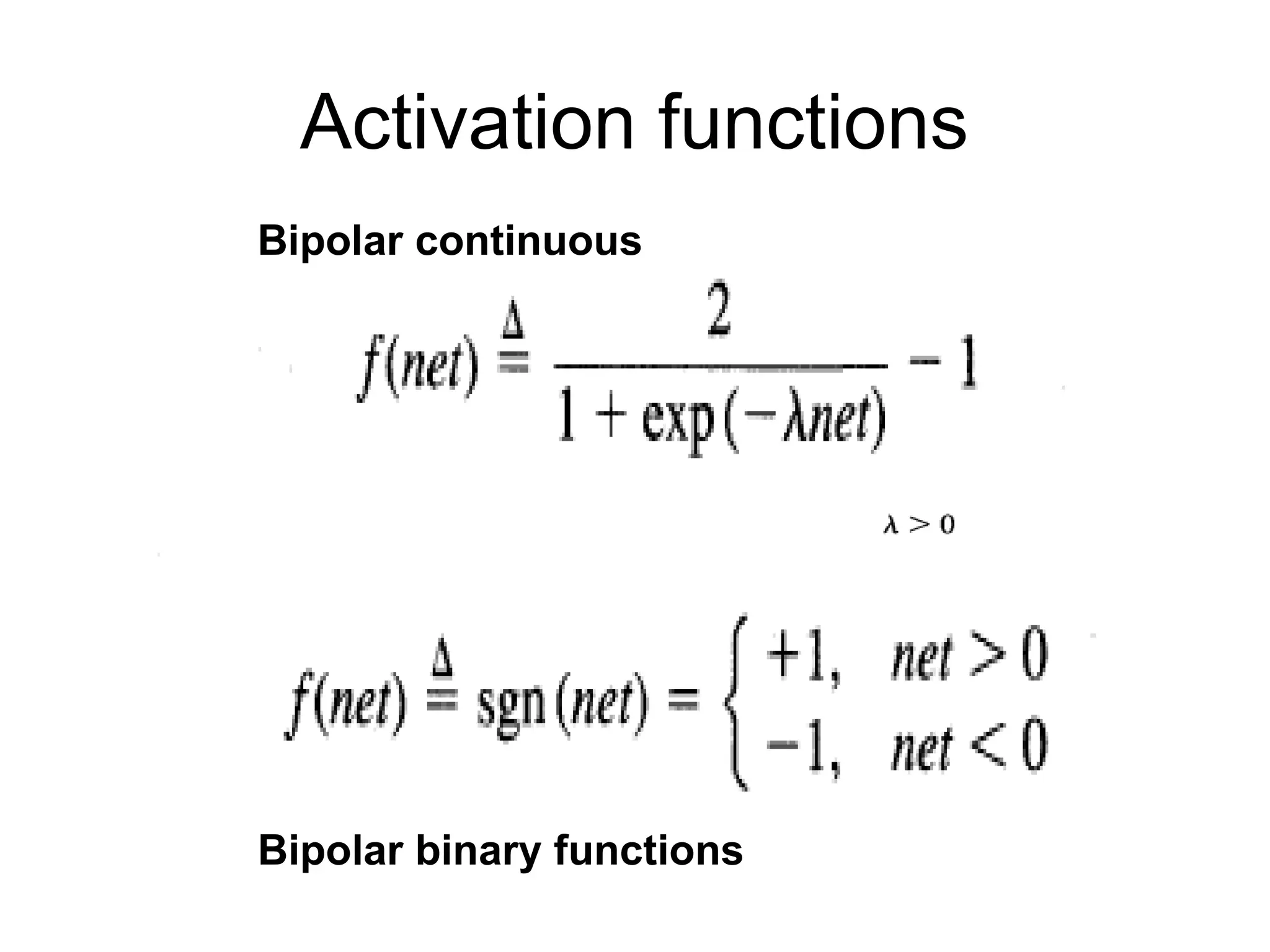
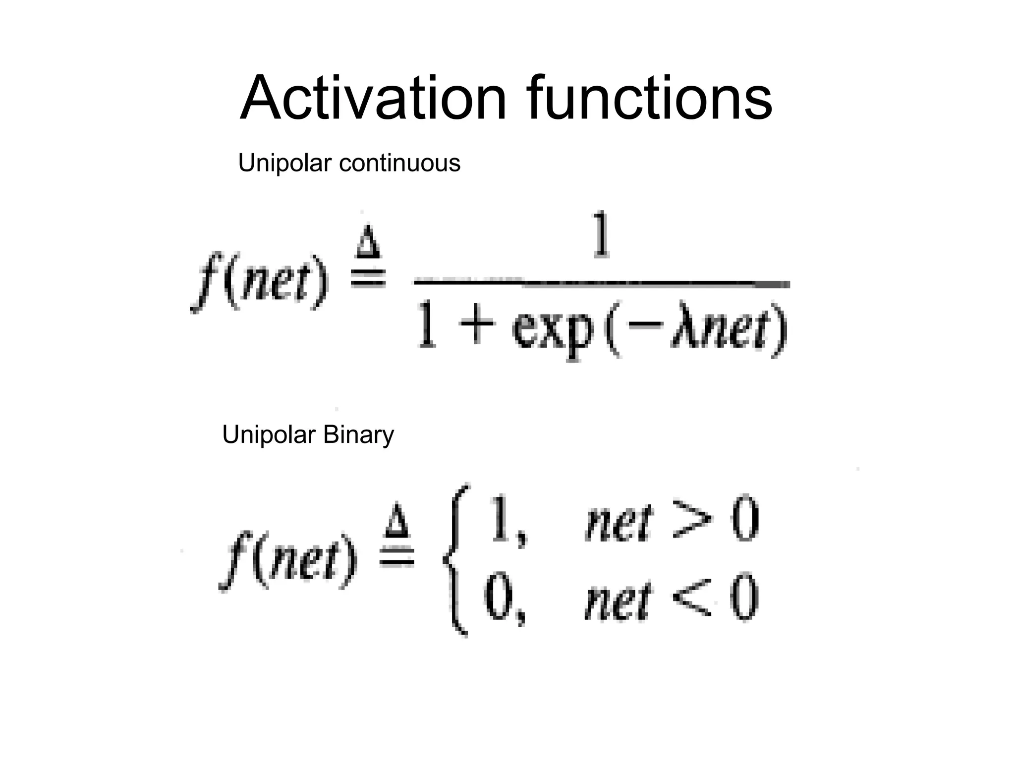
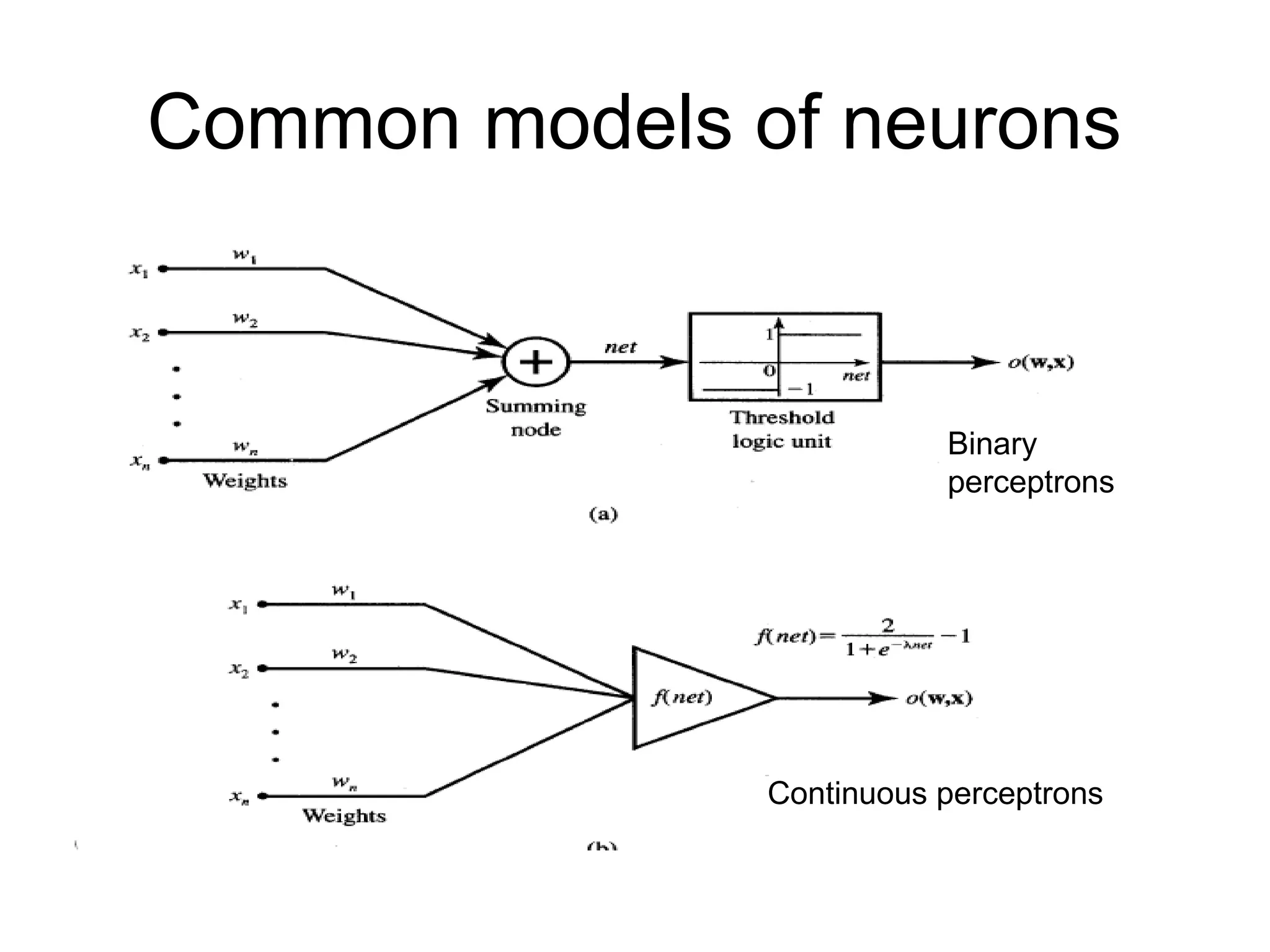
Activation function • Bipolar binary and unipolar binary are called as hard limiting activation functions used in discrete neuron model • Unipolar continuous and bipolar continuous are called soft limiting activation functions are called sigmoidal characteristics.

Activation functions Bipolar continuous Bipolar binary functions

Activation functions Unipolar continuous Unipolar Binary

Common models of neurons Binary perceptrons Continuous perceptrons

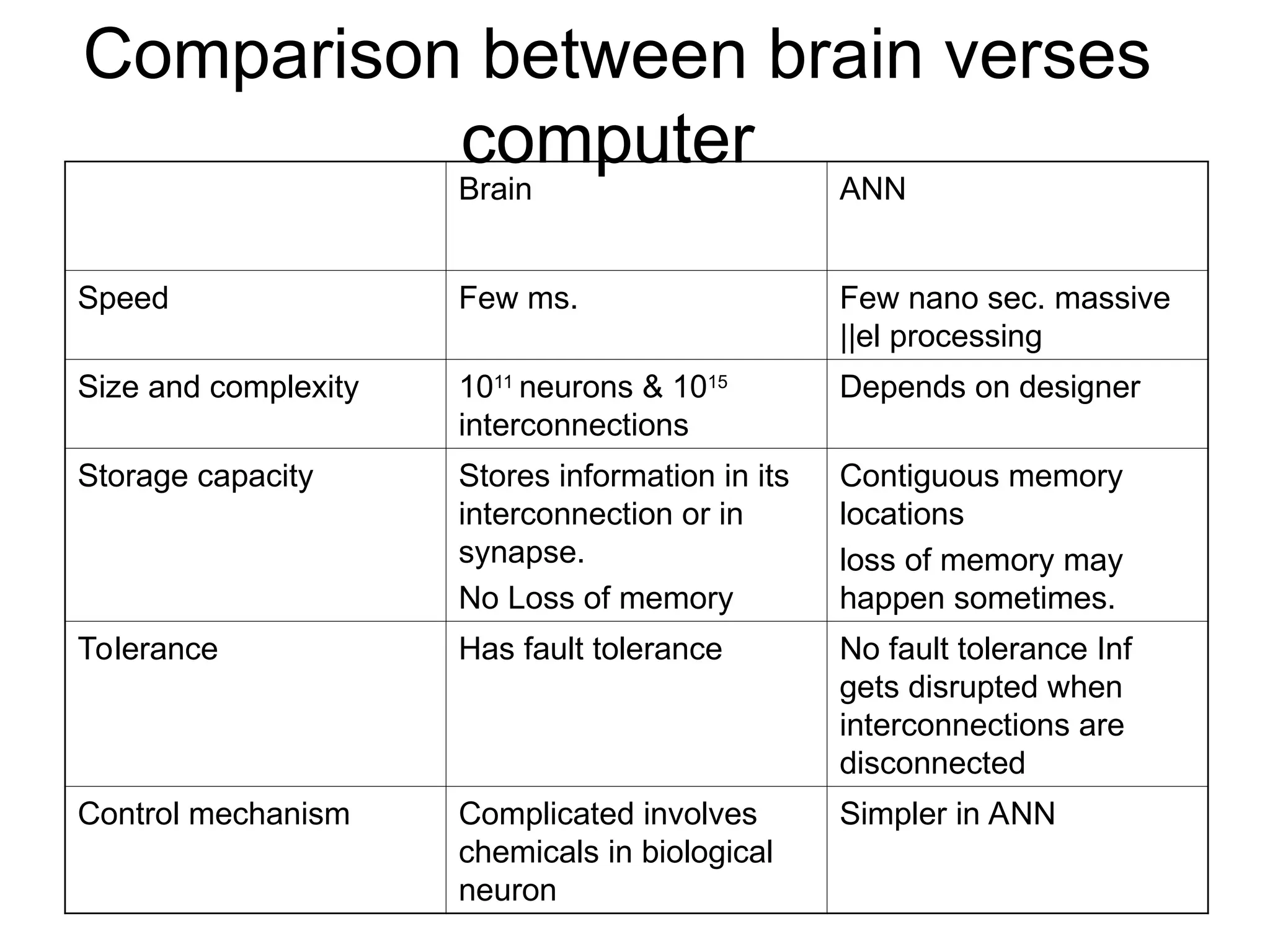
Comparison between brain verses computer Brain ANN Speed Few ms. Few nano sec. massive ||el processing Size and complexity 1011 neurons & 1015 interconnections Depends on designer Storage capacity Stores information in its interconnection or in synapse. No Loss of memory Contiguous memory locations loss of memory may happen sometimes. Tolerance Has fault tolerance No fault tolerance Inf gets disrupted when interconnections are disconnected Control mechanism Complicated involves chemicals in biological neuron Simpler in ANN

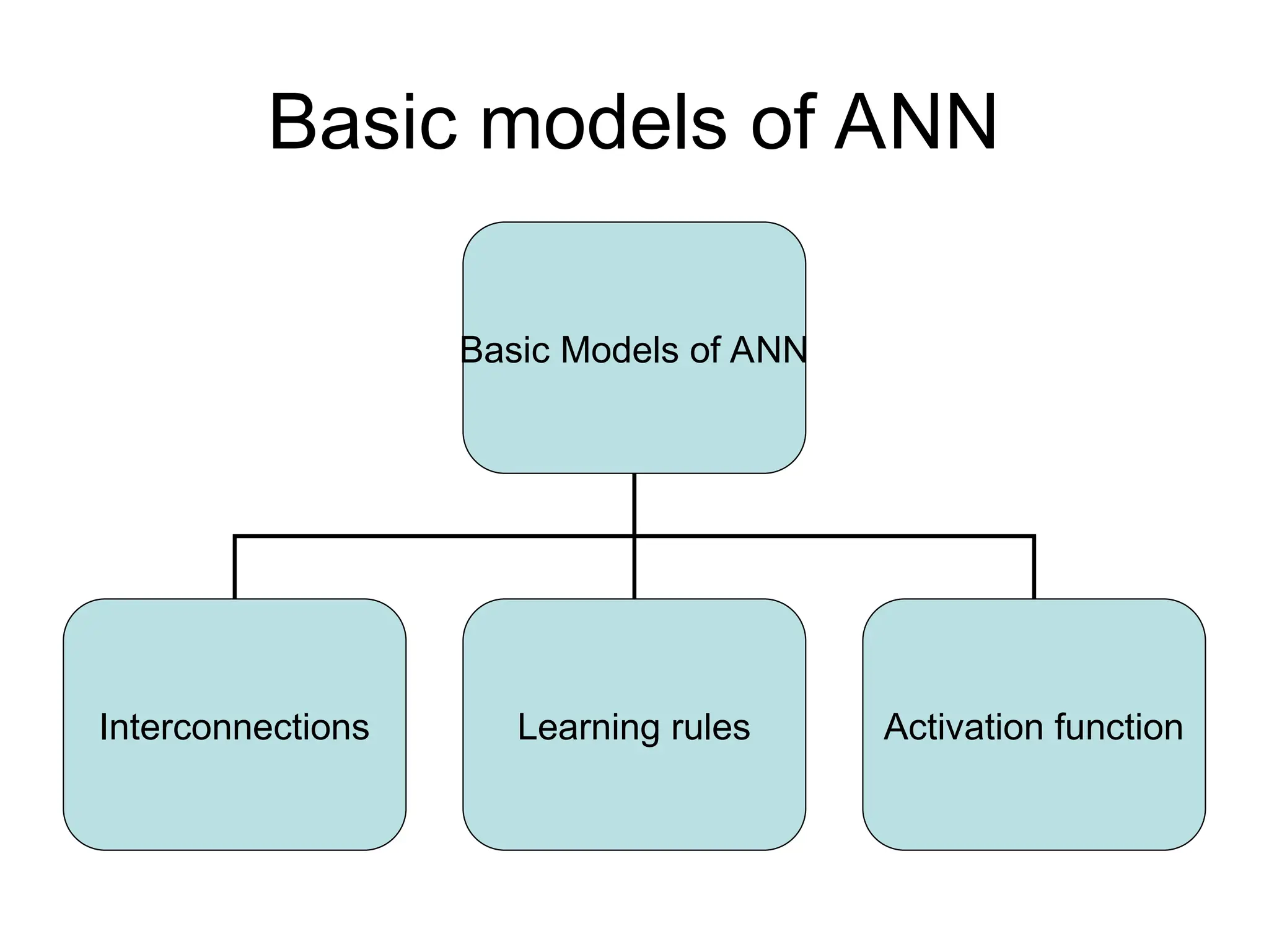
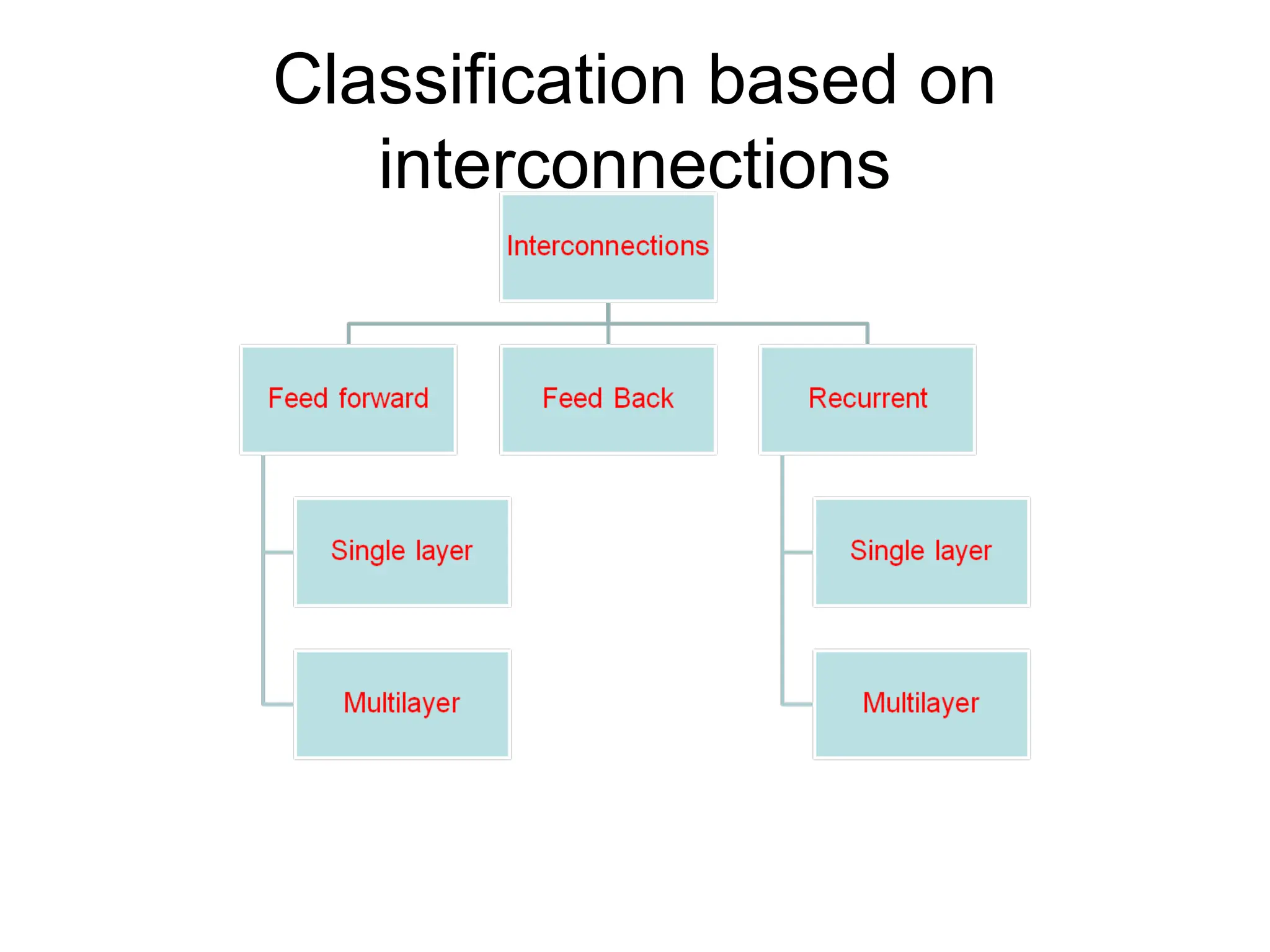
Basic models of ANN Basic Models of ANN Interconnections Learning rules Activation function

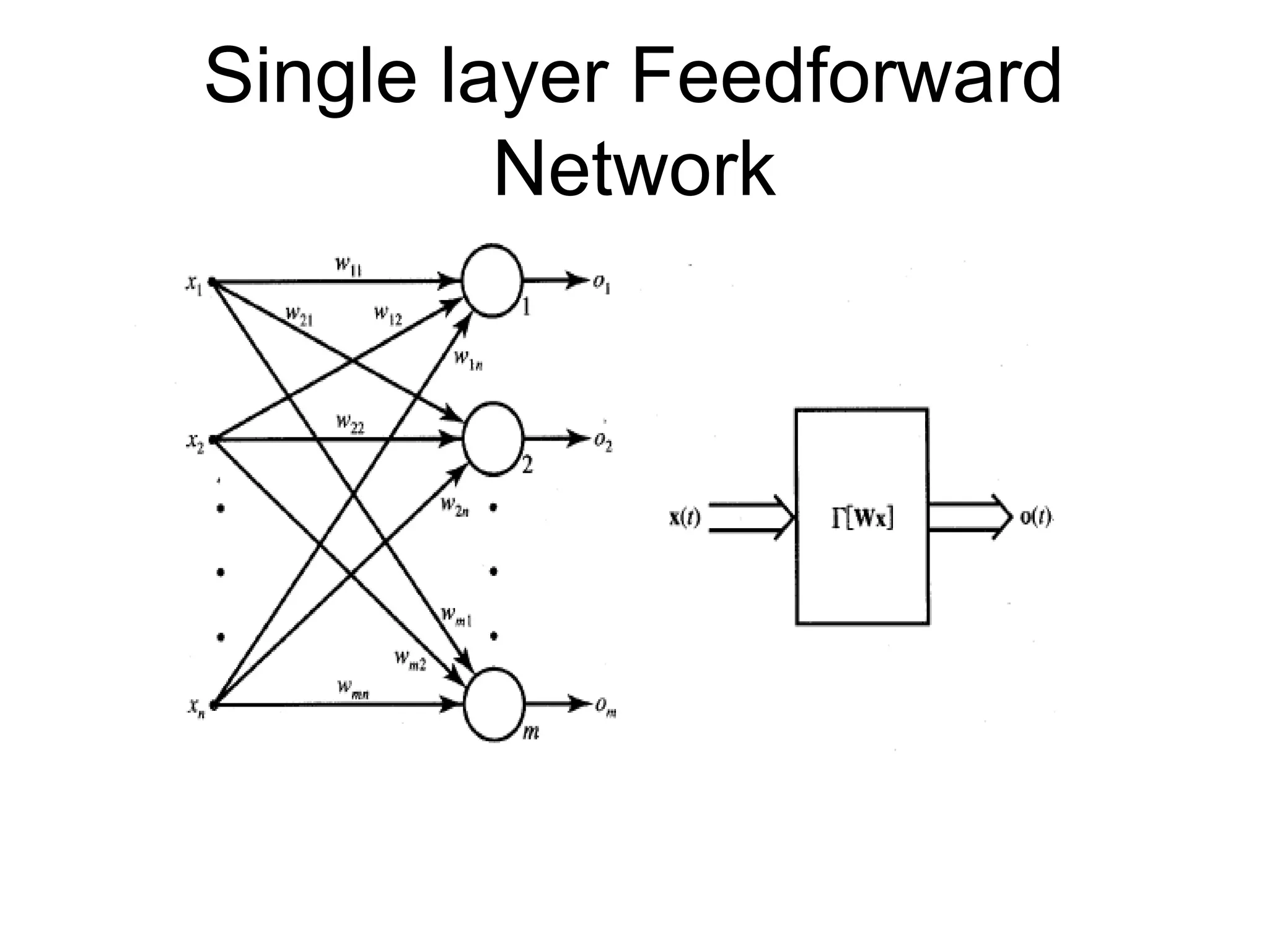
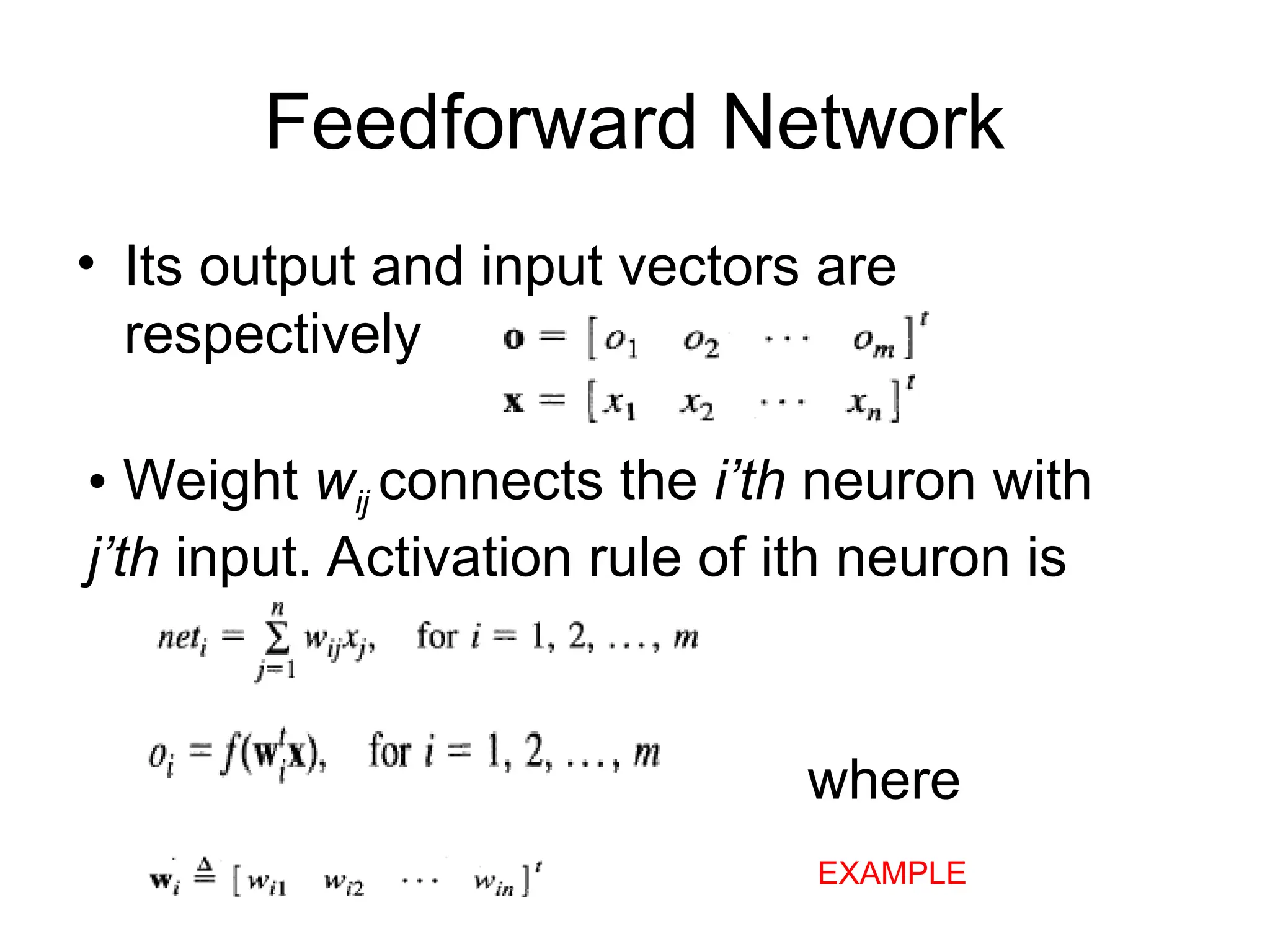
Classification based on interconnections

Single layer Feedforward Network

Feedforward Network • Its output and input vectors are respectively • Weight wij connects the i’th neuron with j’th input. Activation rule of ith neuron is where EXAMPLE

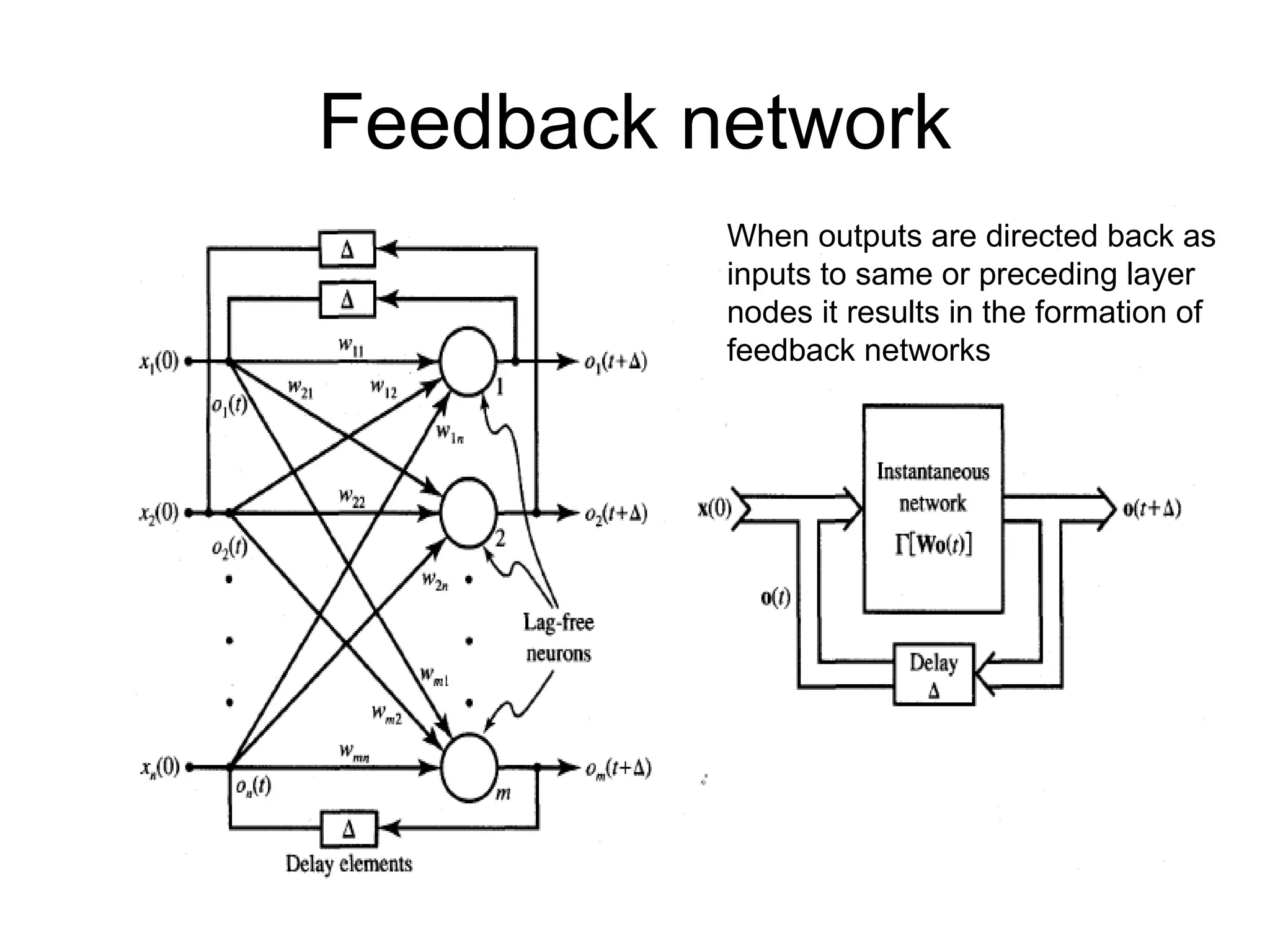
Multilayer feed forward network Can be used to solve complicated problems

Feedback network When outputs are directed back as inputs to same or preceding layer nodes it results in the formation of feedback networks

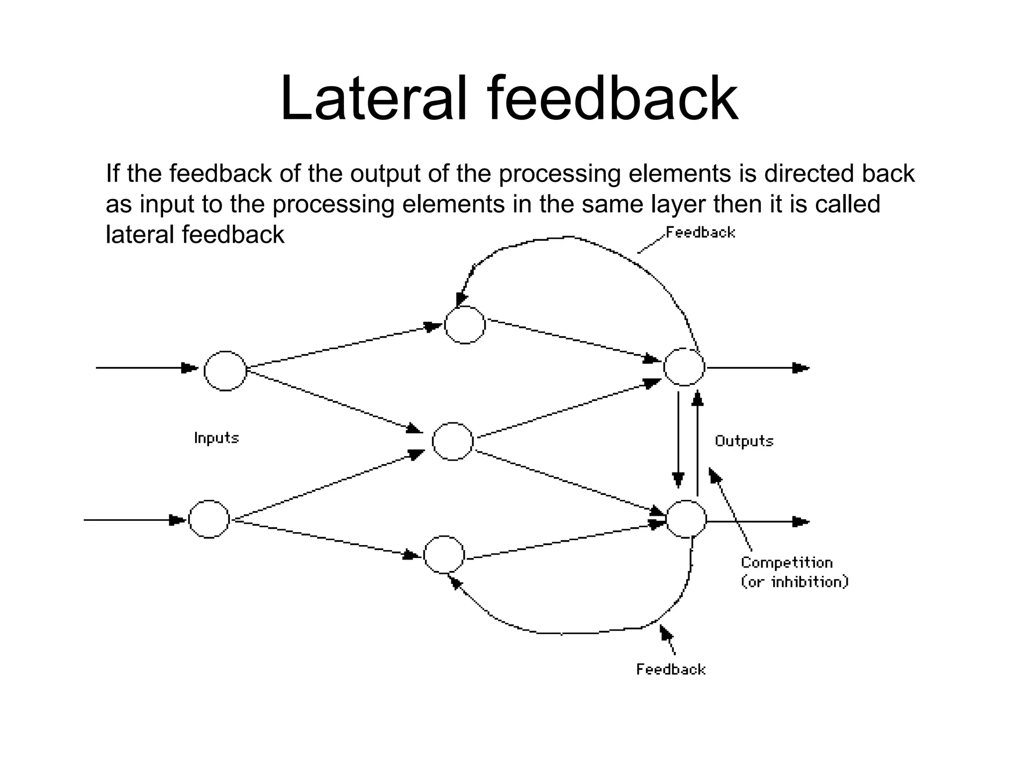
Lateral feedback If the feedback of the output of the processing elements is directed back as input to the processing elements in the same layer then it is called lateral feedback

Recurrent n/ws • Single node with own feedback • Competitive nets • Single-layer recurrent nts • Multilayer recurrent networks Feedback networks with closed loop are called Recurrent Networks. The response at the k+1’th instant depends on the entire history of the network starting at k=0. Automaton: A system with discrete time inputs and a discrete data representation is called an automaton

Learning • It’s a process by which a NN adapts itself to a stimulus by making proper parameter adjustments, resulting in the production of desired response • Two kinds of learning – Parameter learning:- connection weights are updated – Structure Learning:- change in network structure

Training • The process of modifying the weights in the connections between network layers with the objective of achieving the expected output is called training a network. • This is achieved through – Supervised learning – Unsupervised learning – Reinforcement learning

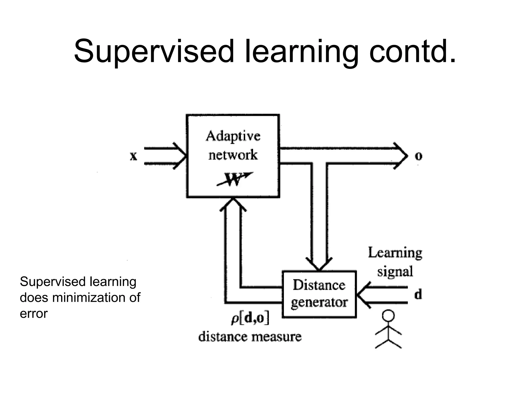
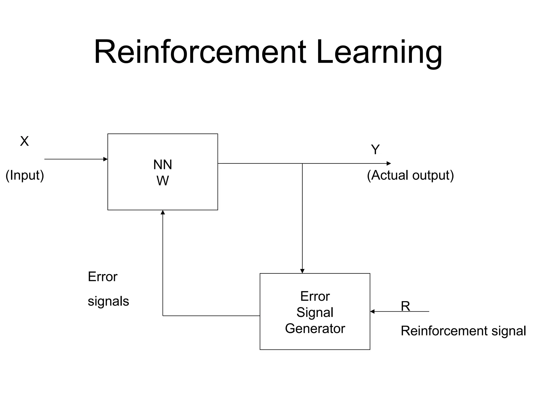
Classification of learning • Supervised learning • Unsupervised learning • Reinforcement learning

Supervised Learning • Child learns from a teacher • Each input vector requires a corresponding target vector. • Training pair=[input vector, target vector] Neural Network W Error Signal Generator X (Input) Y (Actual output) (Desired Output) Error (D-Y) signals

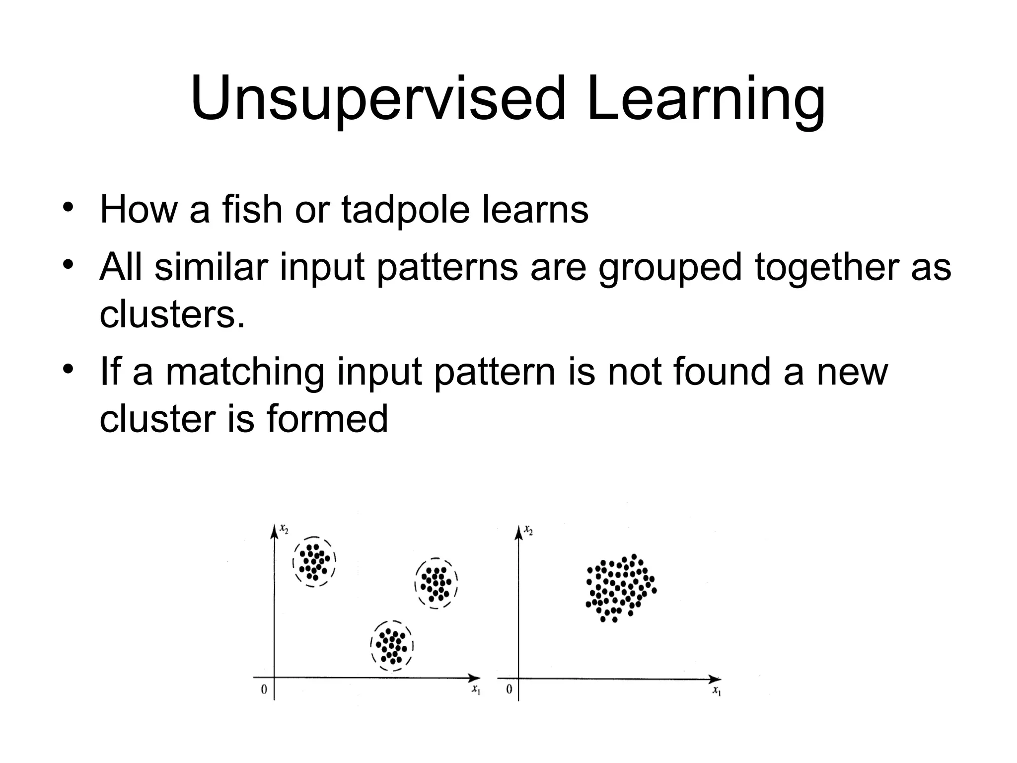
Supervised learning contd. Supervised learning does minimization of error

Unsupervised Learning • How a fish or tadpole learns • All similar input patterns are grouped together as clusters. • If a matching input pattern is not found a new cluster is formed

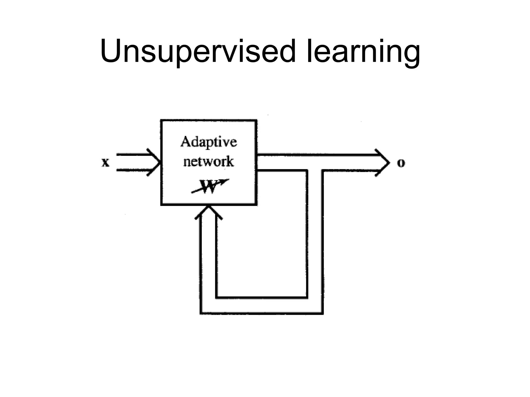
Self-organizing • In unsupervised learning there is no feedback • Network must discover patterns, regularities, features for the input data over the output • While doing so the network might change in parameters • This process is called self-organizing

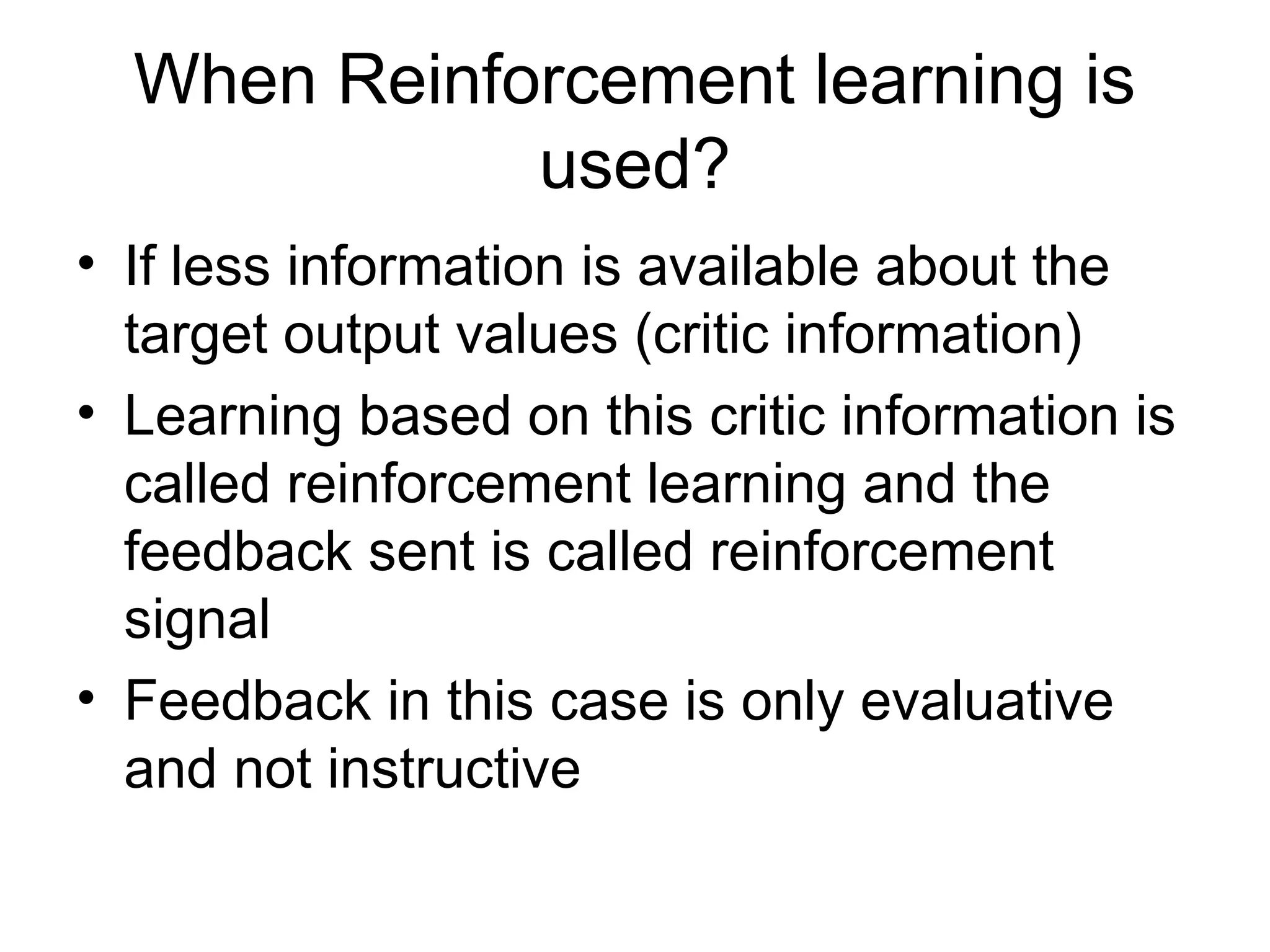
Reinforcement Learning NN W Error Signal Generator X (Input) Y (Actual output) Error signals R Reinforcement signal

When Reinforcement learning is used? • If less information is available about the target output values (critic information) • Learning based on this critic information is called reinforcement learning and the feedback sent is called reinforcement signal • Feedback in this case is only evaluative and not instructive

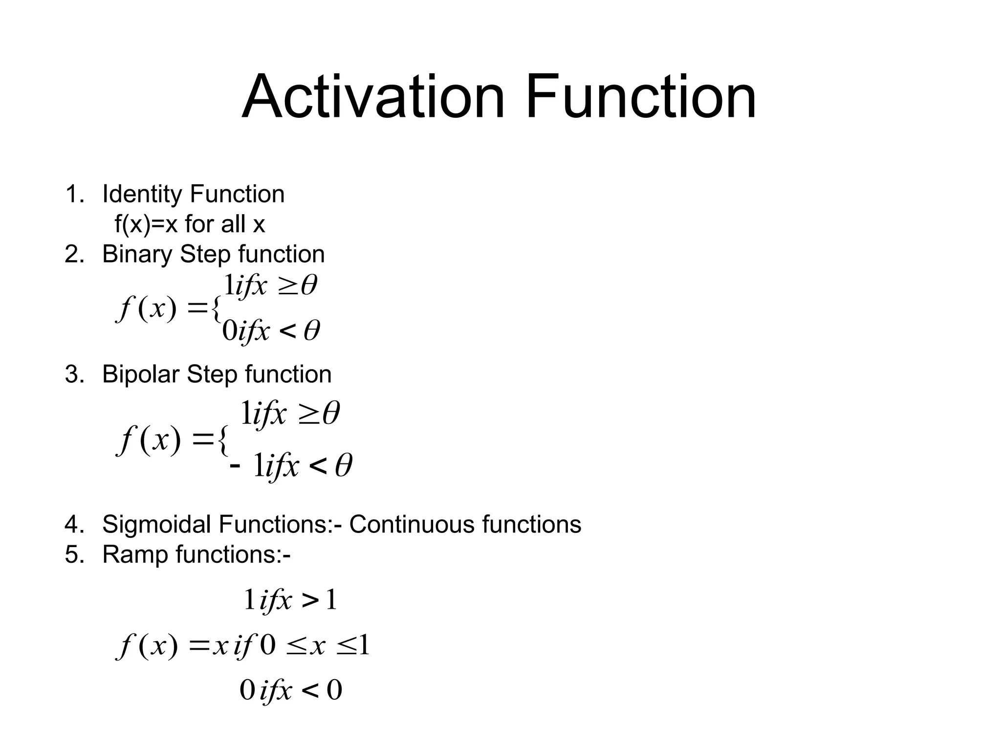
1. Identity Function f(x)=x for all x 2. Binary Step function 3. Bipolar Step function 4. Sigmoidal Functions:- Continuous functions 5. Ramp functions:- Activation Function      ifx ifx x f 0 1 { ) (       ifx ifx x f 1 1 { ) ( 0 0 1 0 1 1 ) (      ifx x if x ifx x f

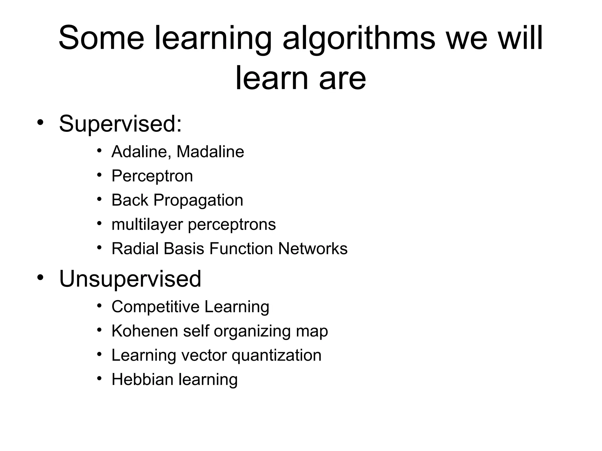
Some learning algorithms we will learn are • Supervised: • Adaline, Madaline • Perceptron • Back Propagation • multilayer perceptrons • Radial Basis Function Networks • Unsupervised • Competitive Learning • Kohenen self organizing map • Learning vector quantization • Hebbian learning

Neural processing • Recall:- processing phase for a NN and its objective is to retrieve the information. The process of computing o for a given x • Basic forms of neural information processing – Auto association – Hetero association – Classification

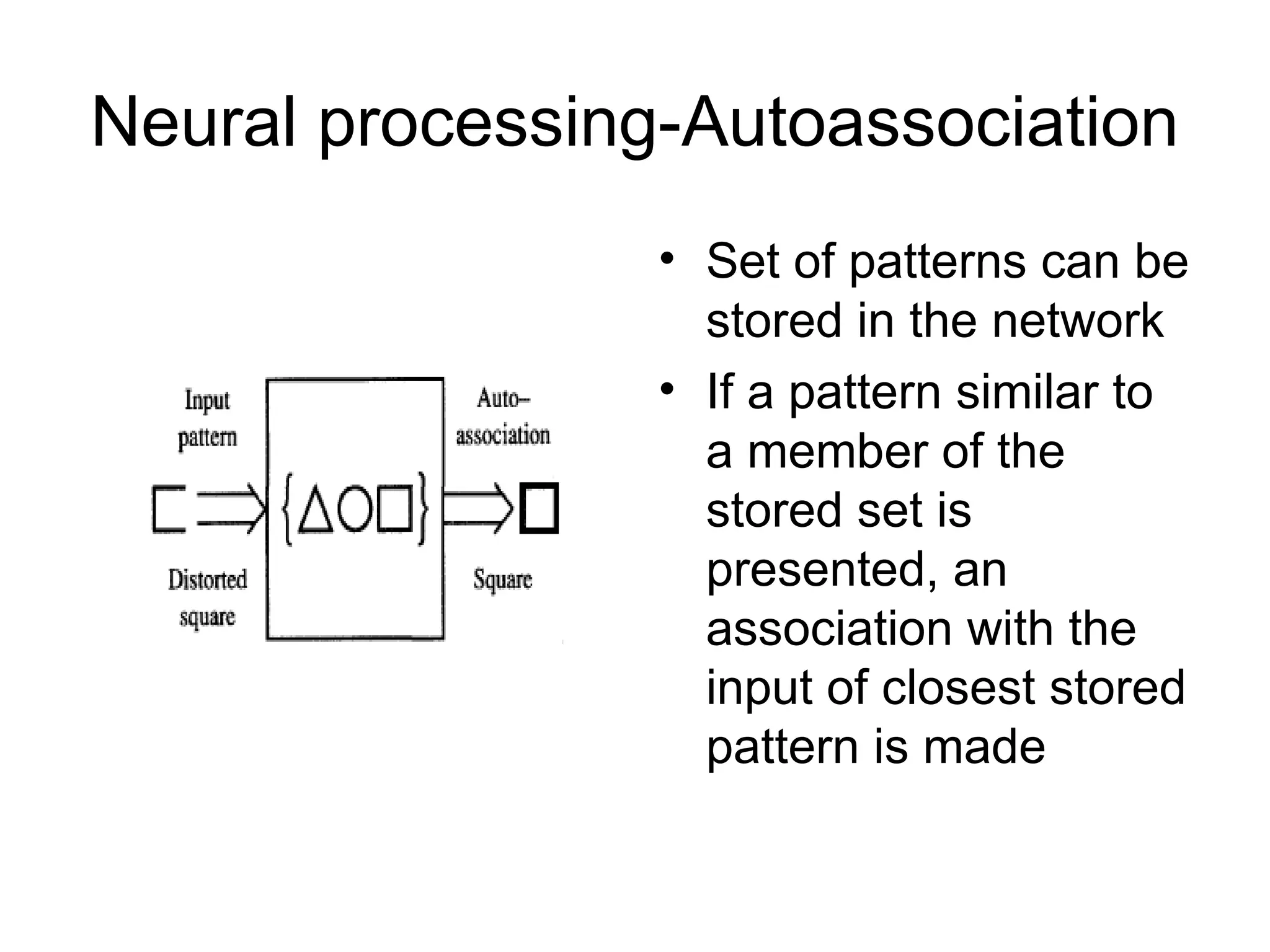
Neural processing-Autoassociation • Set of patterns can be stored in the network • If a pattern similar to a member of the stored set is presented, an association with the input of closest stored pattern is made

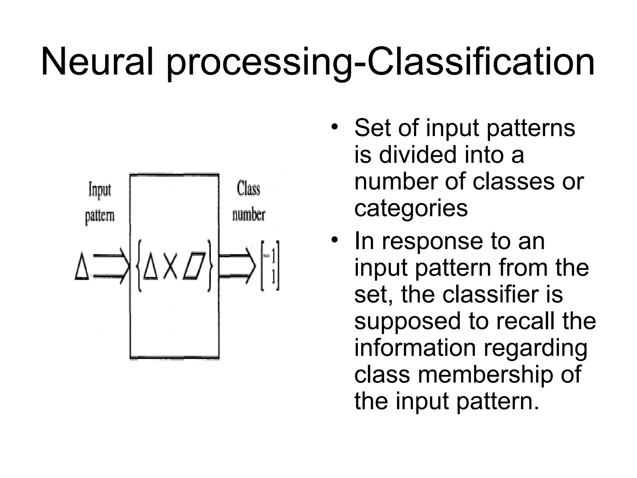
Neural Processing- Heteroassociation • Associations between pairs of patterns are stored • Distorted input pattern may cause correct heteroassociation at the output

Neural processing-Classification • Set of input patterns is divided into a number of classes or categories • In response to an input pattern from the set, the classifier is supposed to recall the information regarding class membership of the input pattern.

Important terminologies of ANNs • Weights • Bias • Threshold • Learning rate • Momentum factor • Vigilance parameter • Notations used in ANN

Weights • Each neuron is connected to every other neuron by means of directed links • Links are associated with weights • Weights contain information about the input signal and is represented as a matrix • Weight matrix also called connection matrix

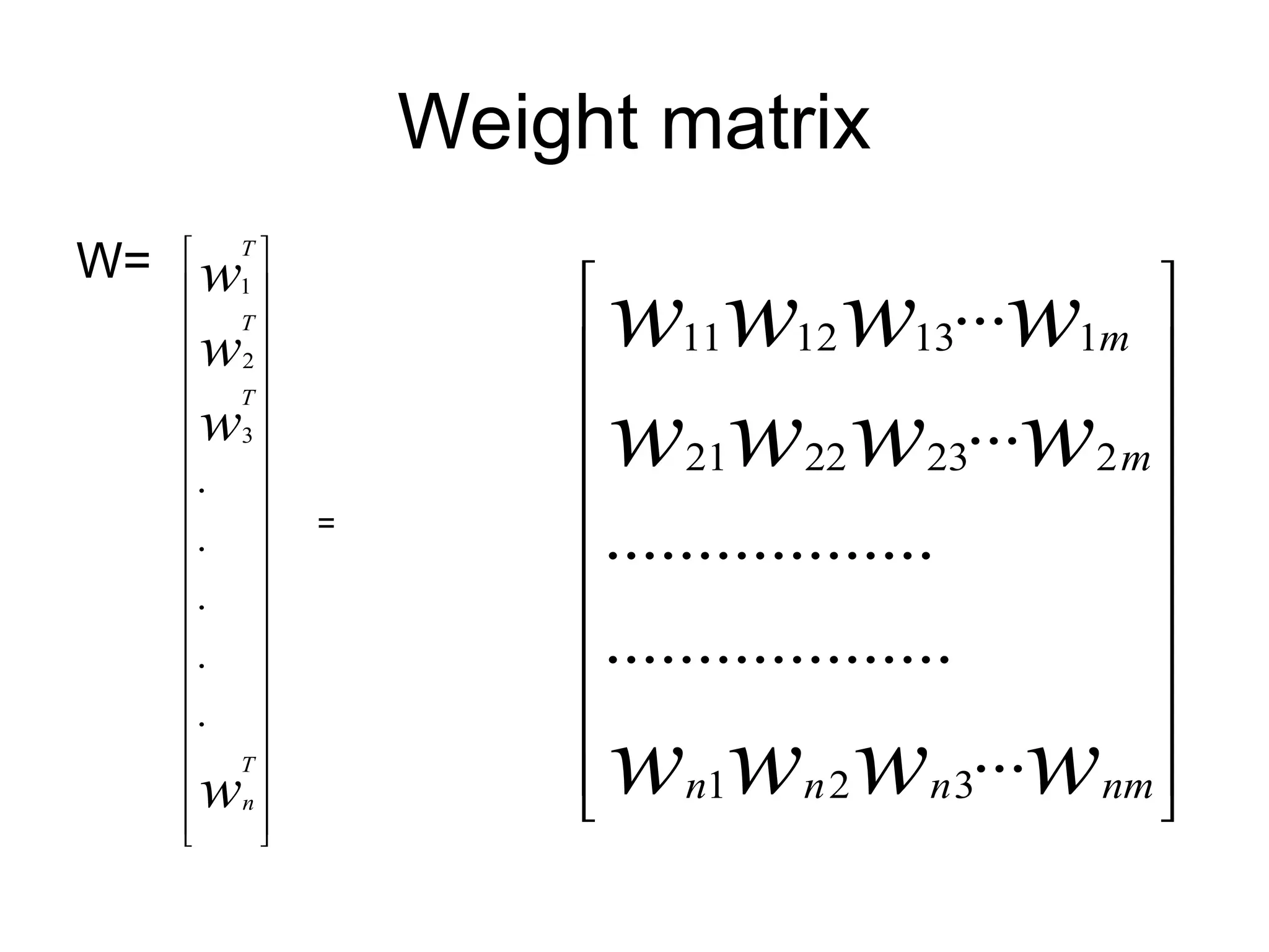
Weight matrix W= 1 2 3 . . . . . T T T T n w w w w                                   = 11 12 13 1 21 22 23 2 1 2 3 ... ... .................. ................... ... m m n n n nm w w w w w w w w w w w w                  

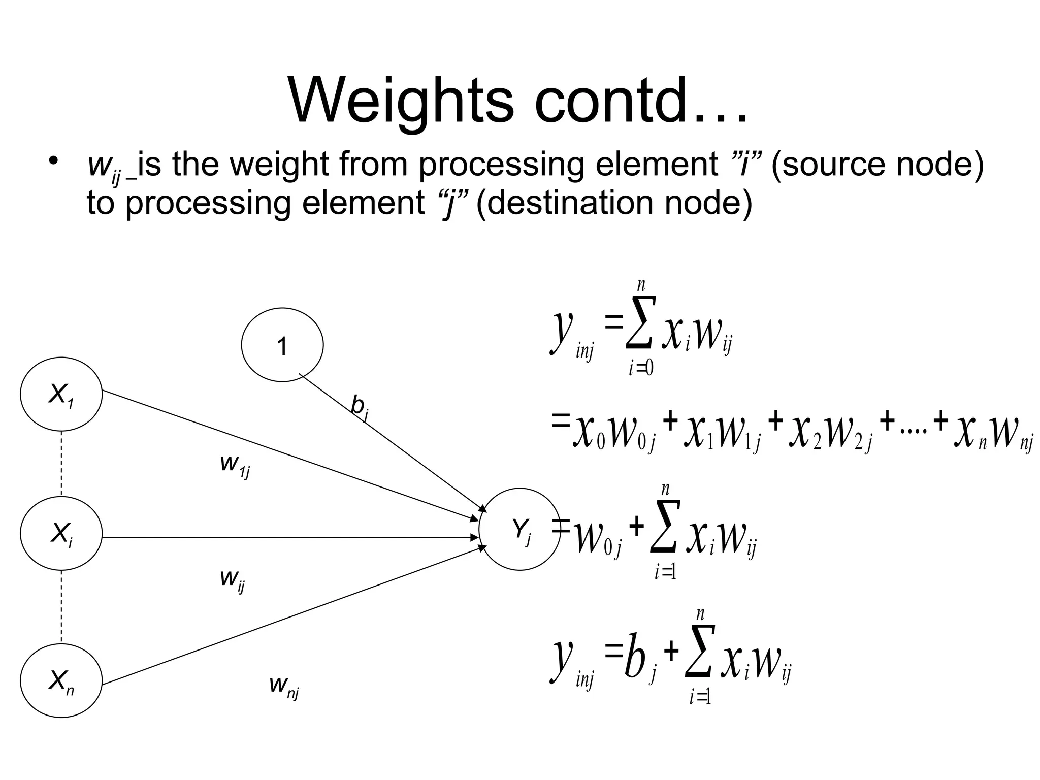
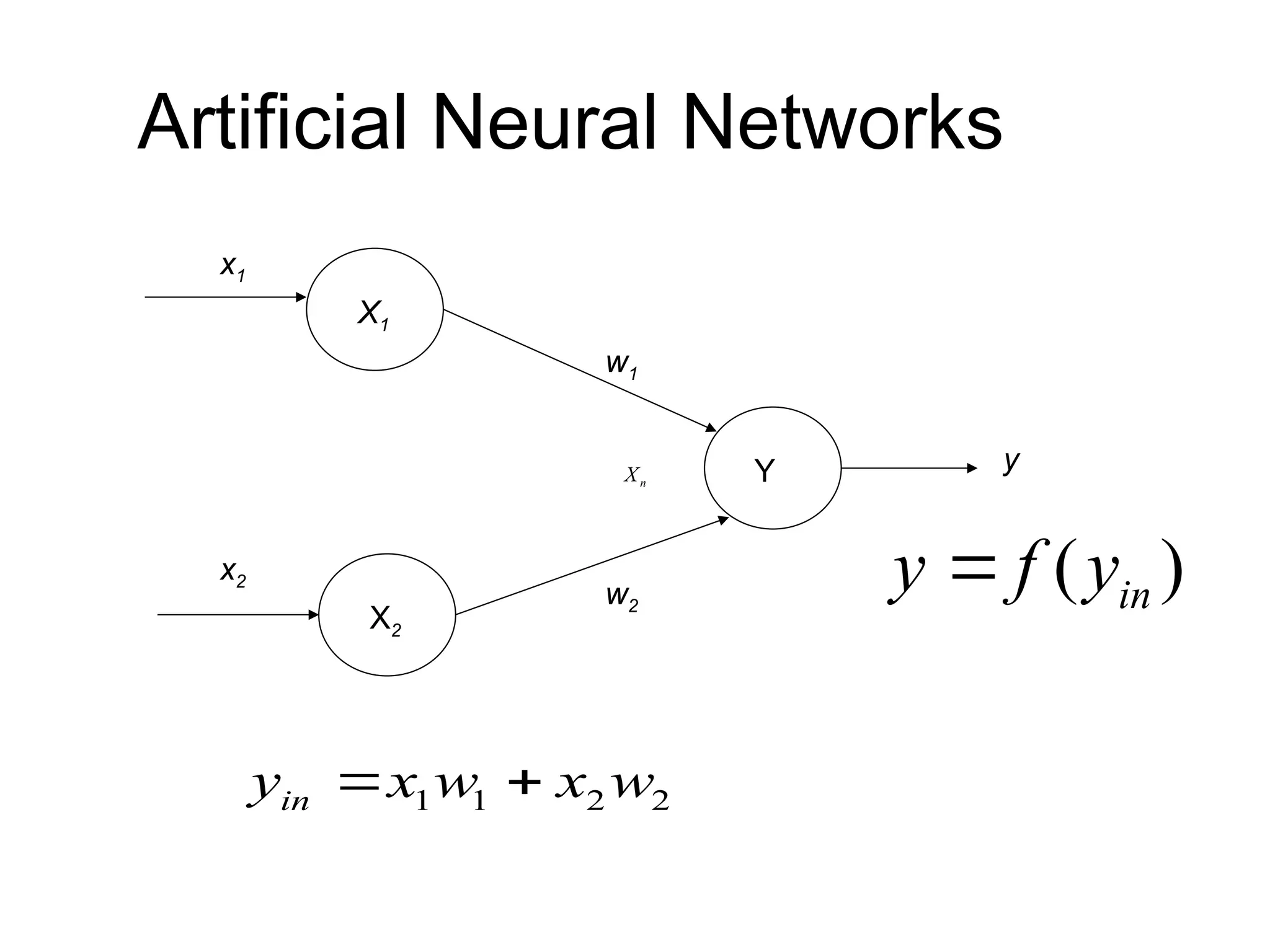
Weights contd… • wij –is the weight from processing element ”i” (source node) to processing element “j” (destination node) X1 1 Xi Yj Xn w1j wij wnj bj 0 0 0 1 1 2 2 0 1 1 .... n i ij inj i j j j n nj n j i ij i n j i ij inj i y xw x w xw x w x w w xw y b xw                

Activation Functions • Used to calculate the output response of a neuron. • Sum of the weighted input signal is applied with an activation to obtain the response. • Activation functions can be linear or non linear • Already dealt – Identity function – Single/binary step function – Discrete/continuous sigmoidal function.

Bias • Bias is like another weight. Its included by adding a component x0=1 to the input vector X. • X=(1,X1,X2…Xi,…Xn) • Bias is of two types – Positive bias: increase the net input – Negative bias: decrease the net input

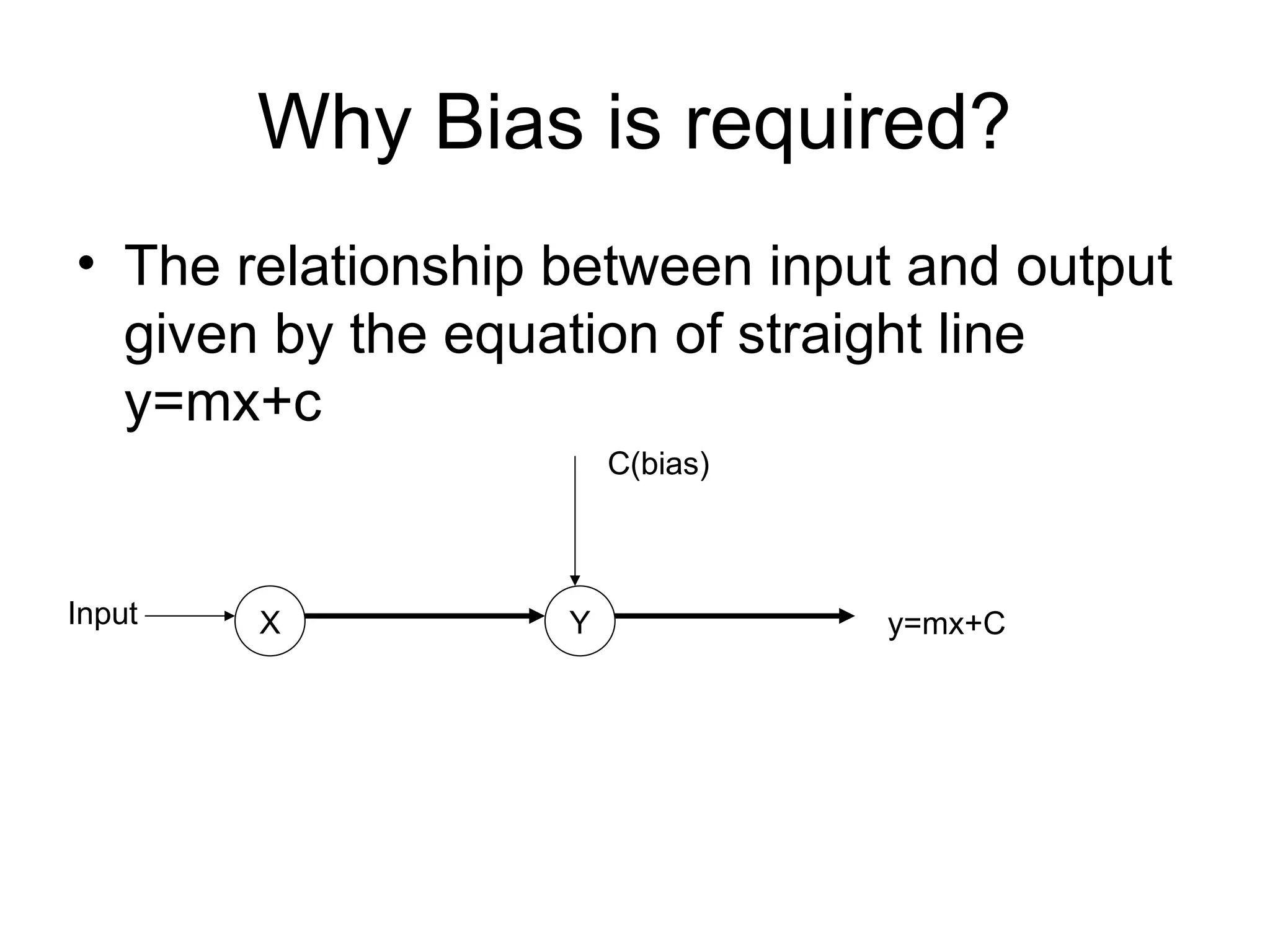
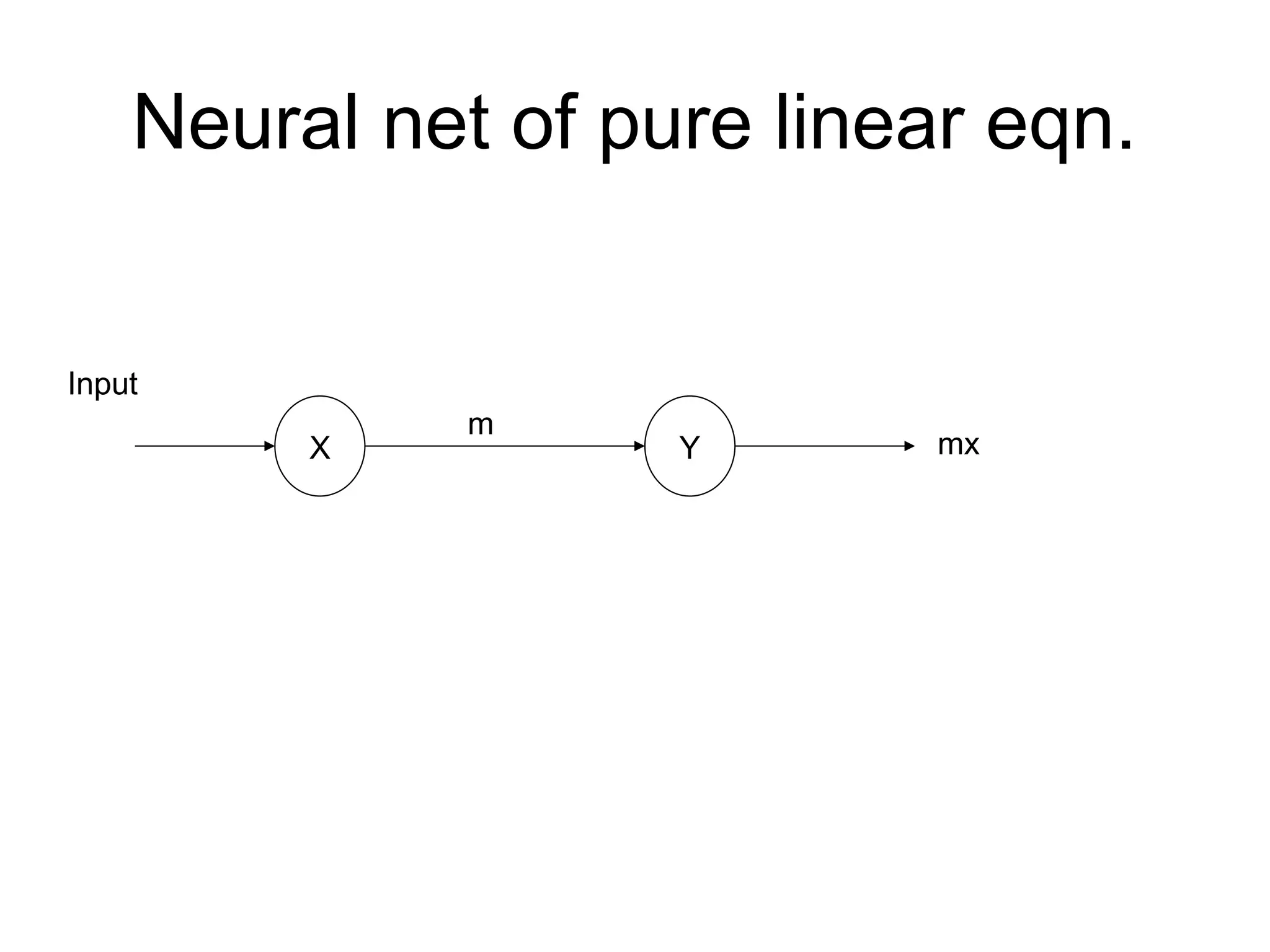
Why Bias is required? • The relationship between input and output given by the equation of straight line y=mx+c X Y Input C(bias) y=mx+C

Threshold • Set value based upon which the final output of the network may be calculated • Used in activation function • The activation function using threshold can be defined as             ifnet ifnet net f 1 1 ) (

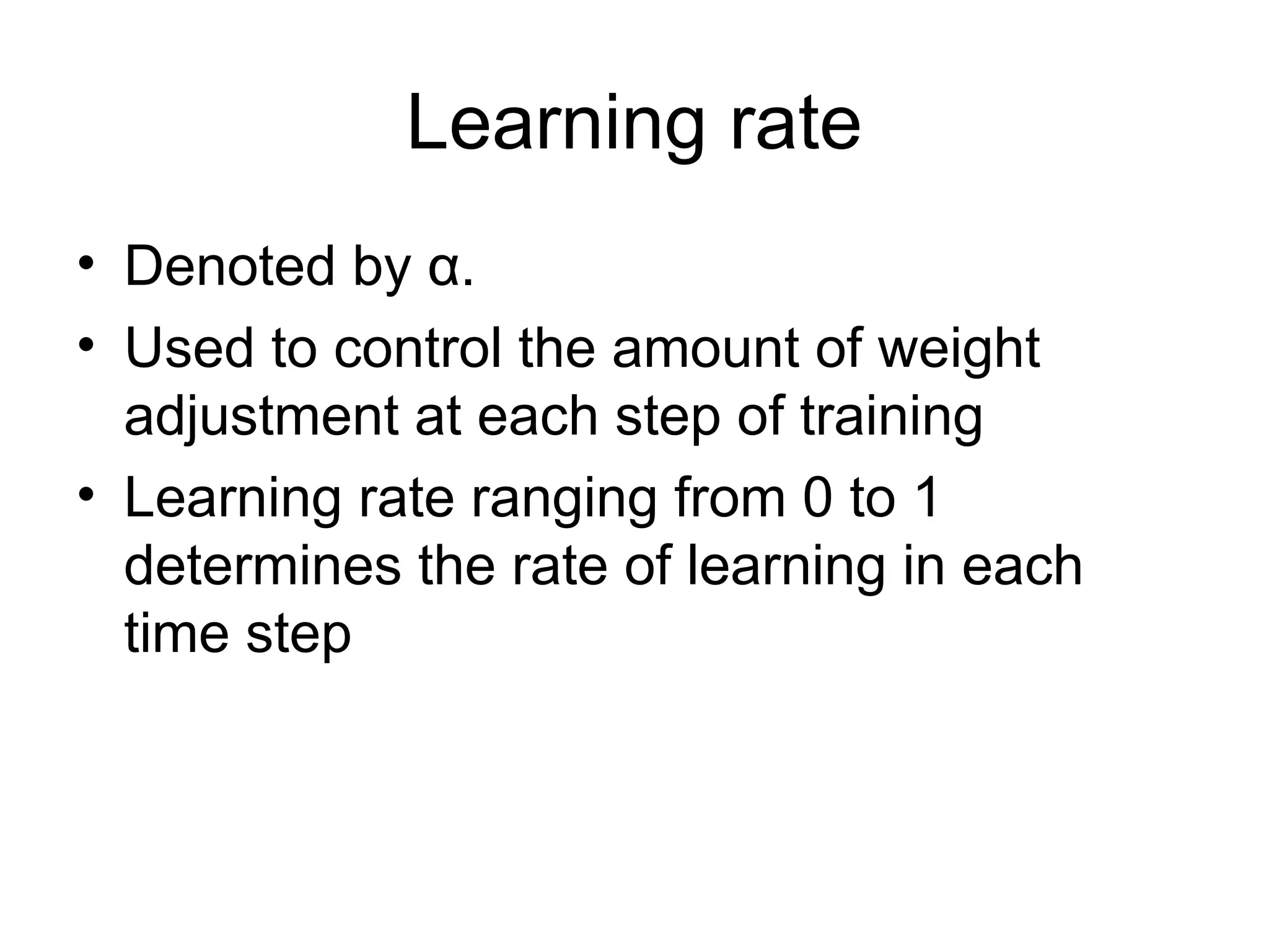
Learning rate • Denoted by α. • Used to control the amount of weight adjustment at each step of training • Learning rate ranging from 0 to 1 determines the rate of learning in each time step

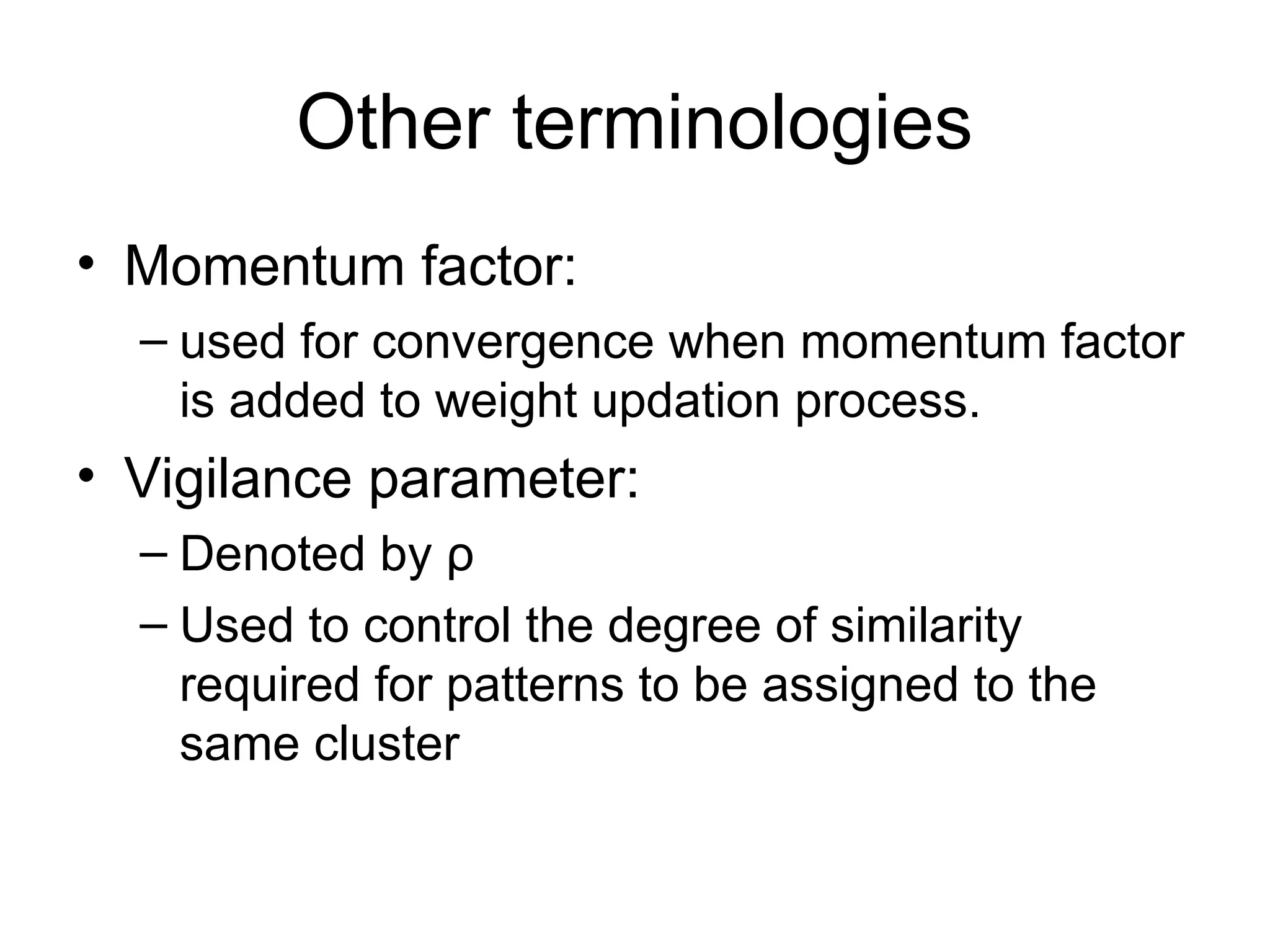
Other terminologies • Momentum factor: – used for convergence when momentum factor is added to weight updation process. • Vigilance parameter: – Denoted by ρ – Used to control the degree of similarity required for patterns to be assigned to the same cluster

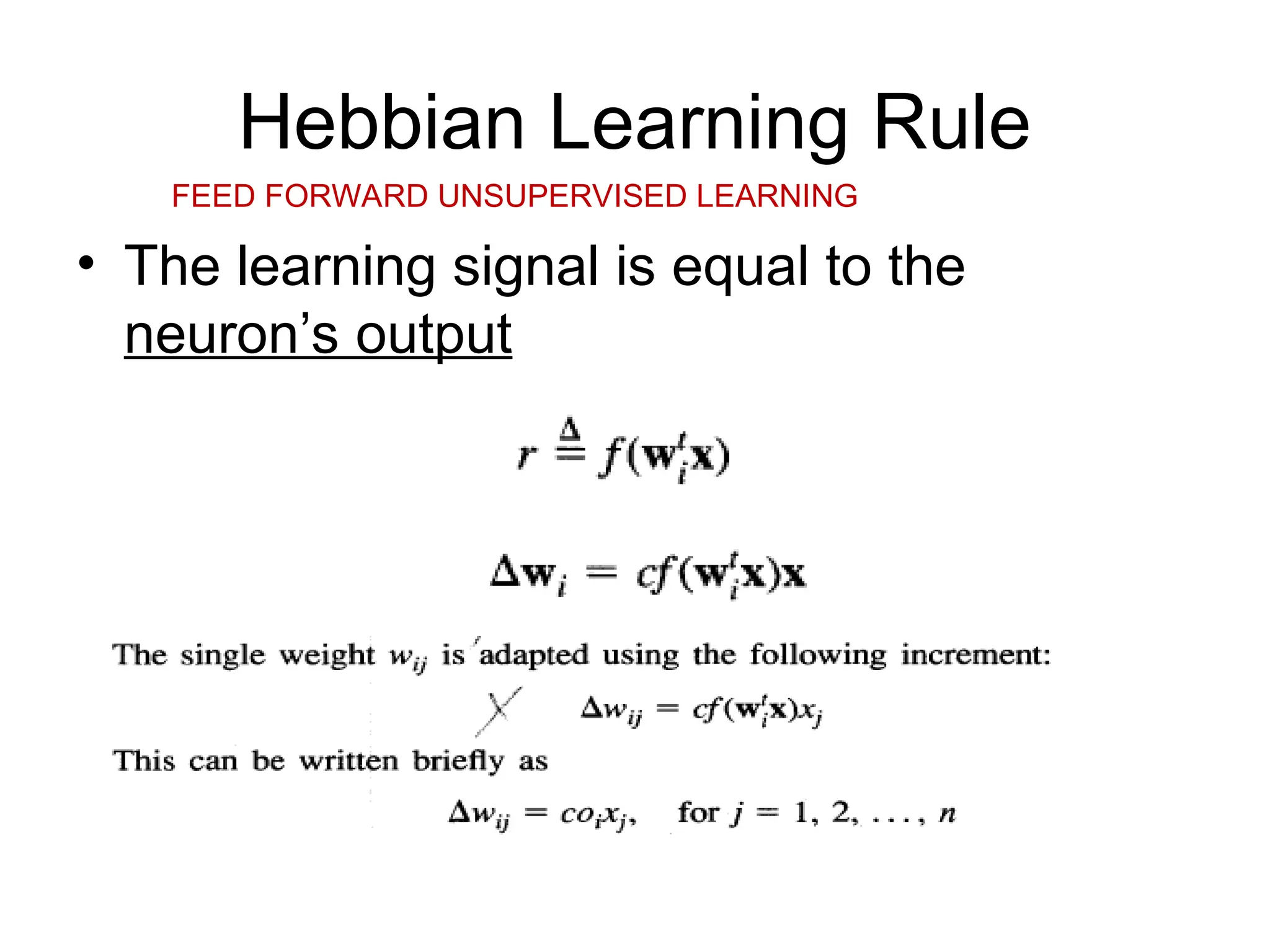
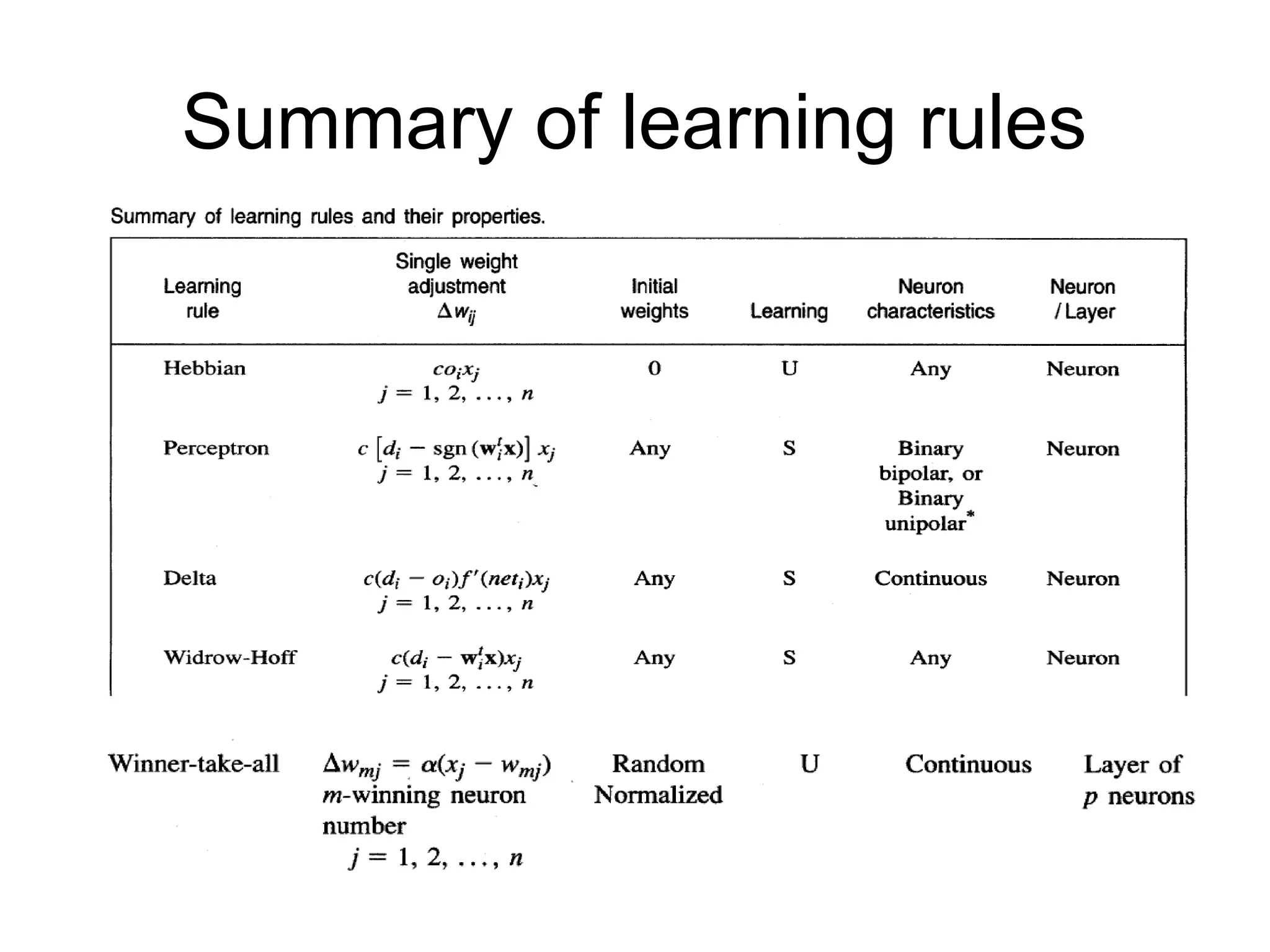
Neural Network Learning rules c – learning constant

Hebbian Learning Rule • The learning signal is equal to the neuron’s output FEED FORWARD UNSUPERVISED LEARNING

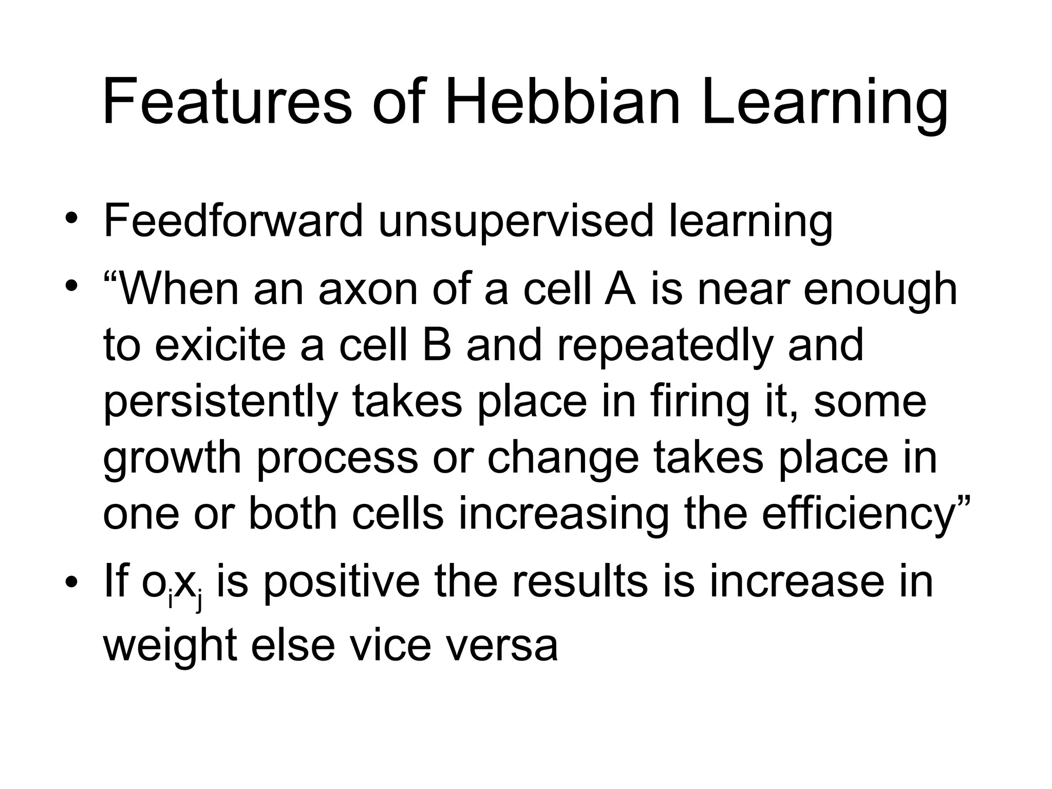
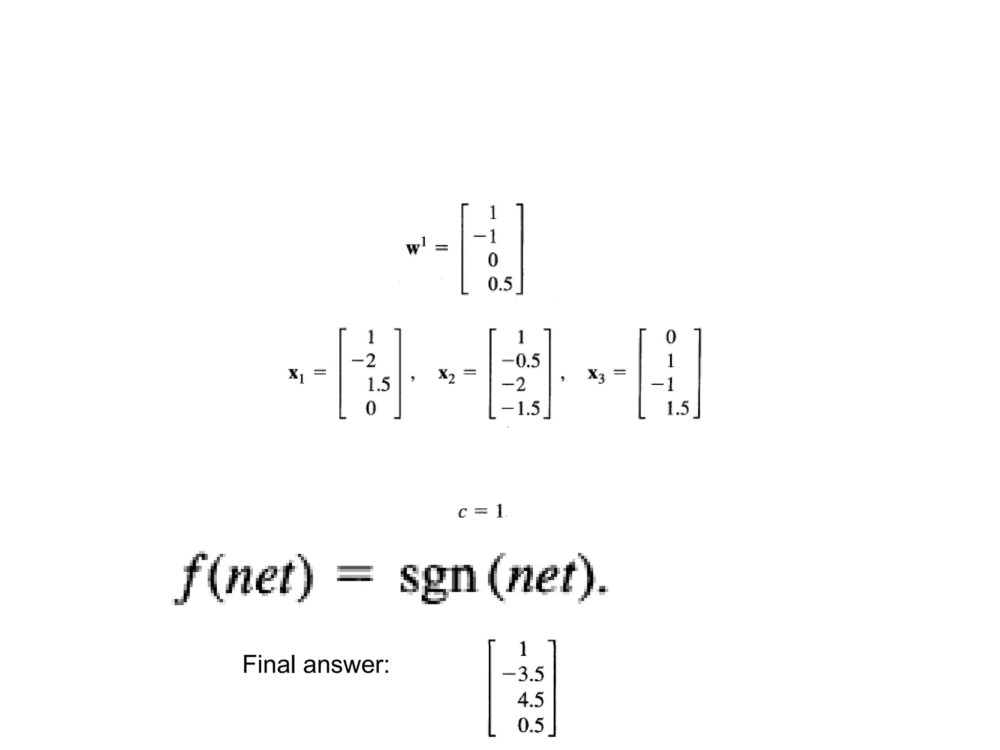
Features of Hebbian Learning • Feedforward unsupervised learning • “When an axon of a cell A is near enough to exicite a cell B and repeatedly and persistently takes place in firing it, some growth process or change takes place in one or both cells increasing the efficiency” • If oixj is positive the results is increase in weight else vice versa

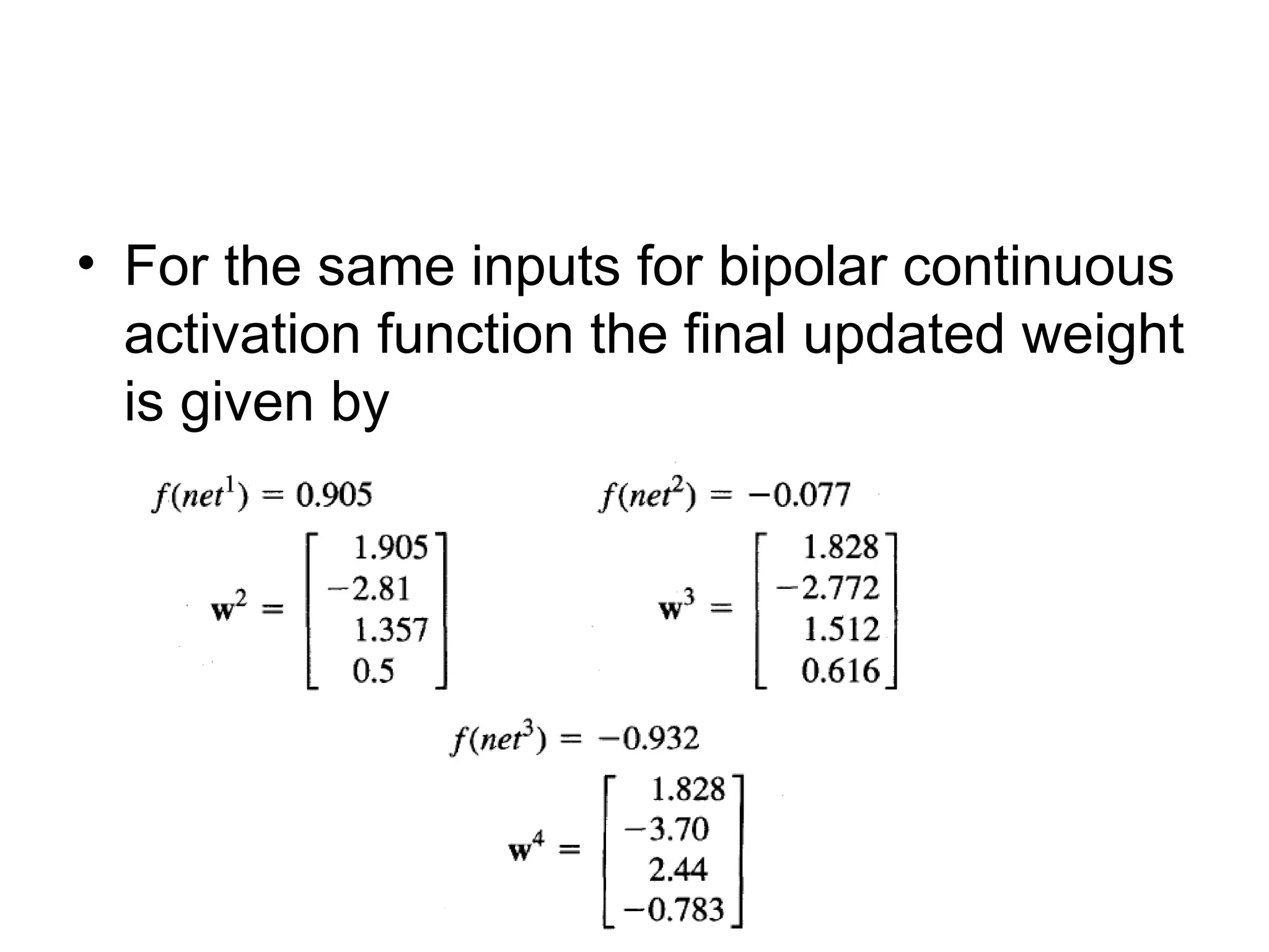
• For the same inputs for bipolar continuous activation function the final updated weight is given by

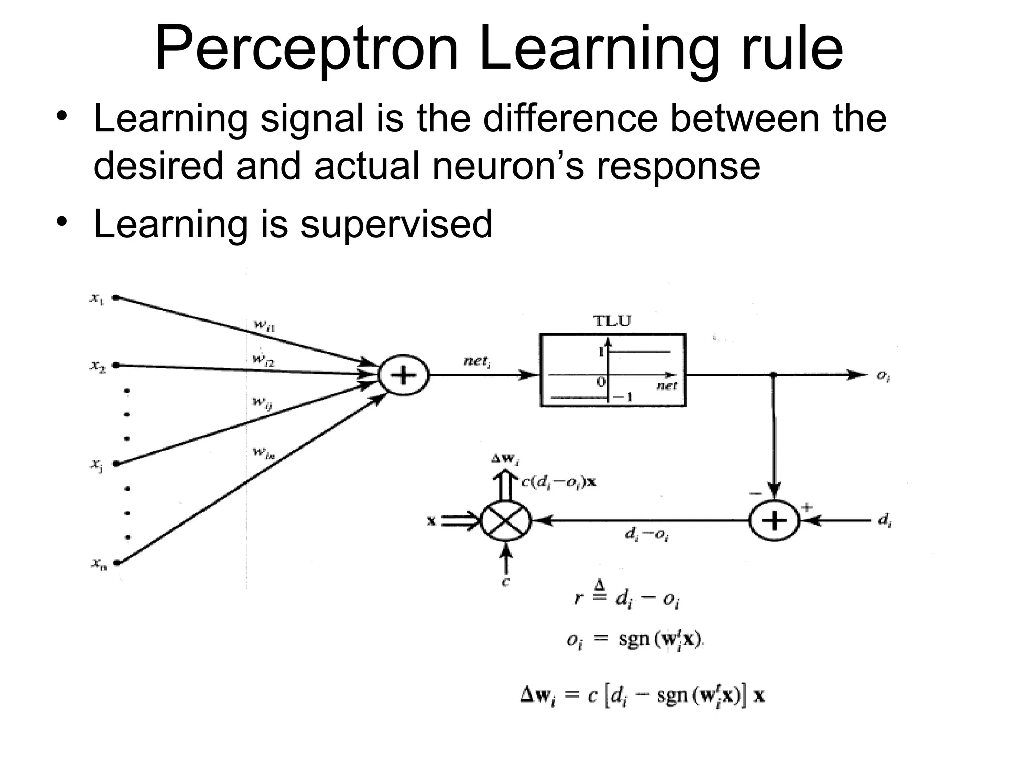
Perceptron Learning rule • Learning signal is the difference between the desired and actual neuron’s response • Learning is supervised

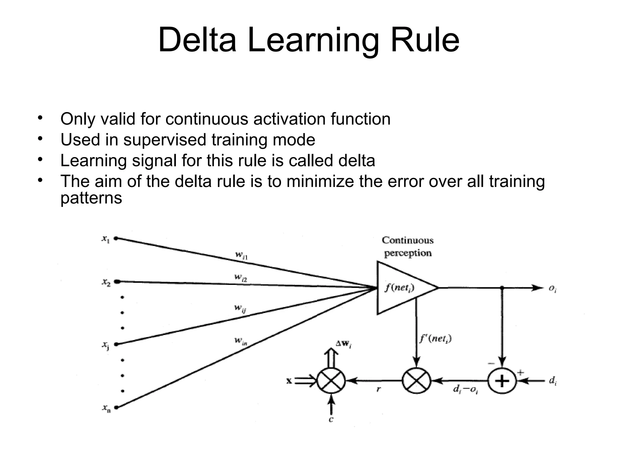
Delta Learning Rule • Only valid for continuous activation function • Used in supervised training mode • Learning signal for this rule is called delta • The aim of the delta rule is to minimize the error over all training patterns

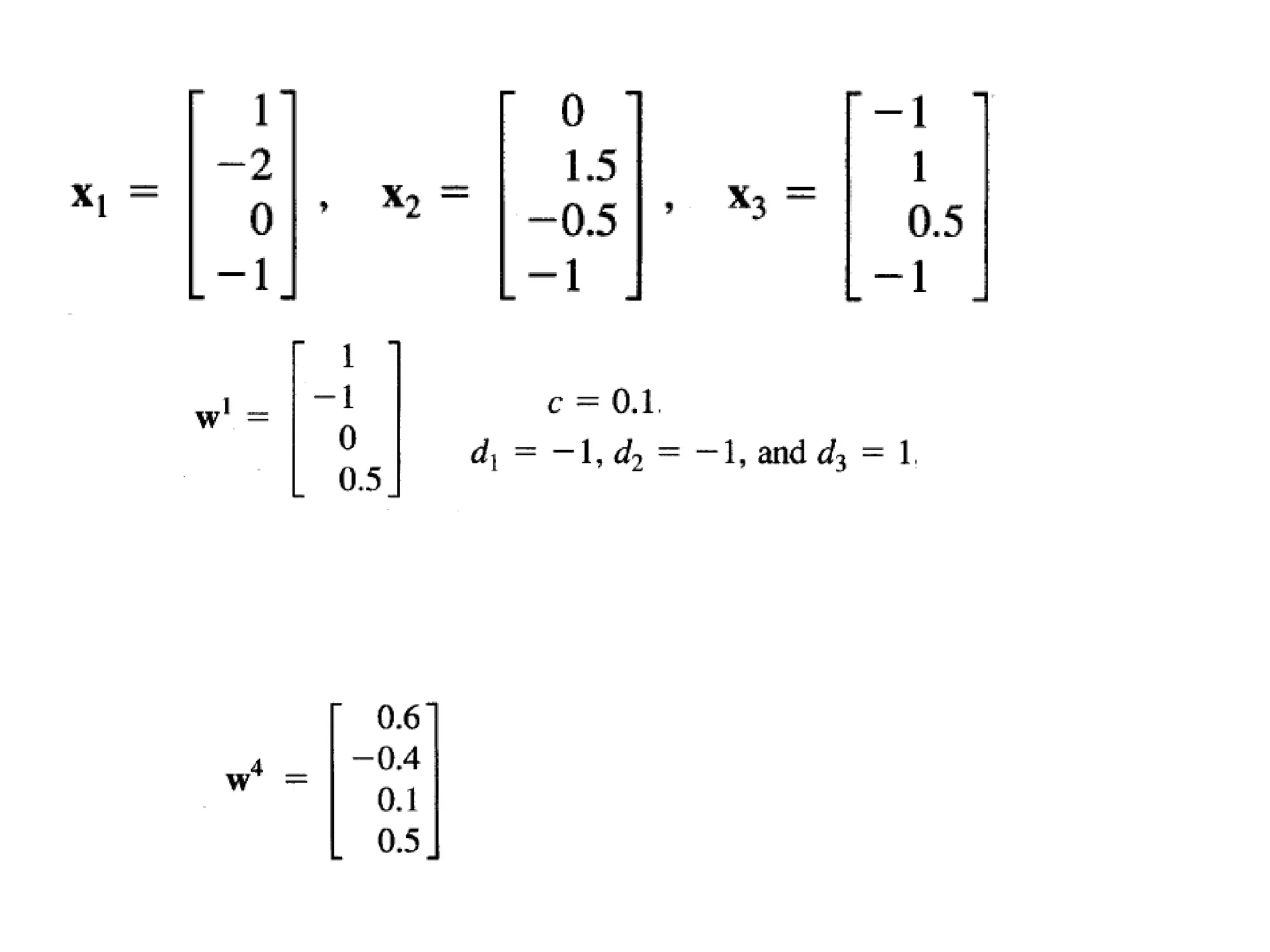
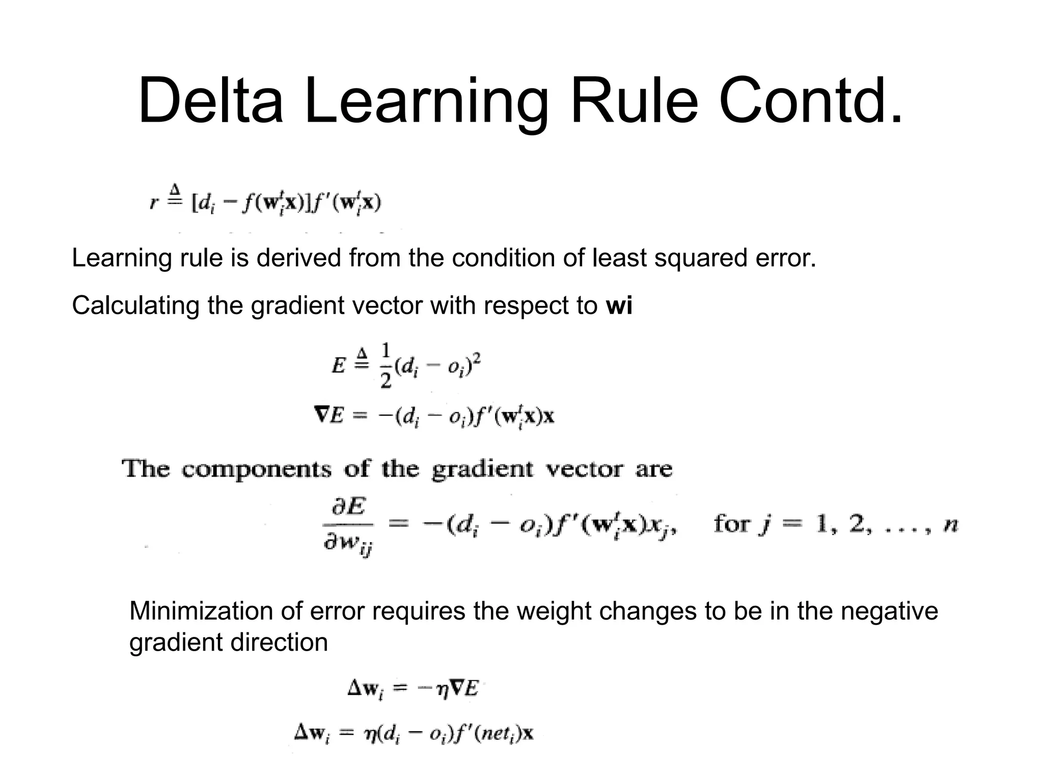
Delta Learning Rule Contd. Learning rule is derived from the condition of least squared error. Calculating the gradient vector with respect to wi Minimization of error requires the weight changes to be in the negative gradient direction

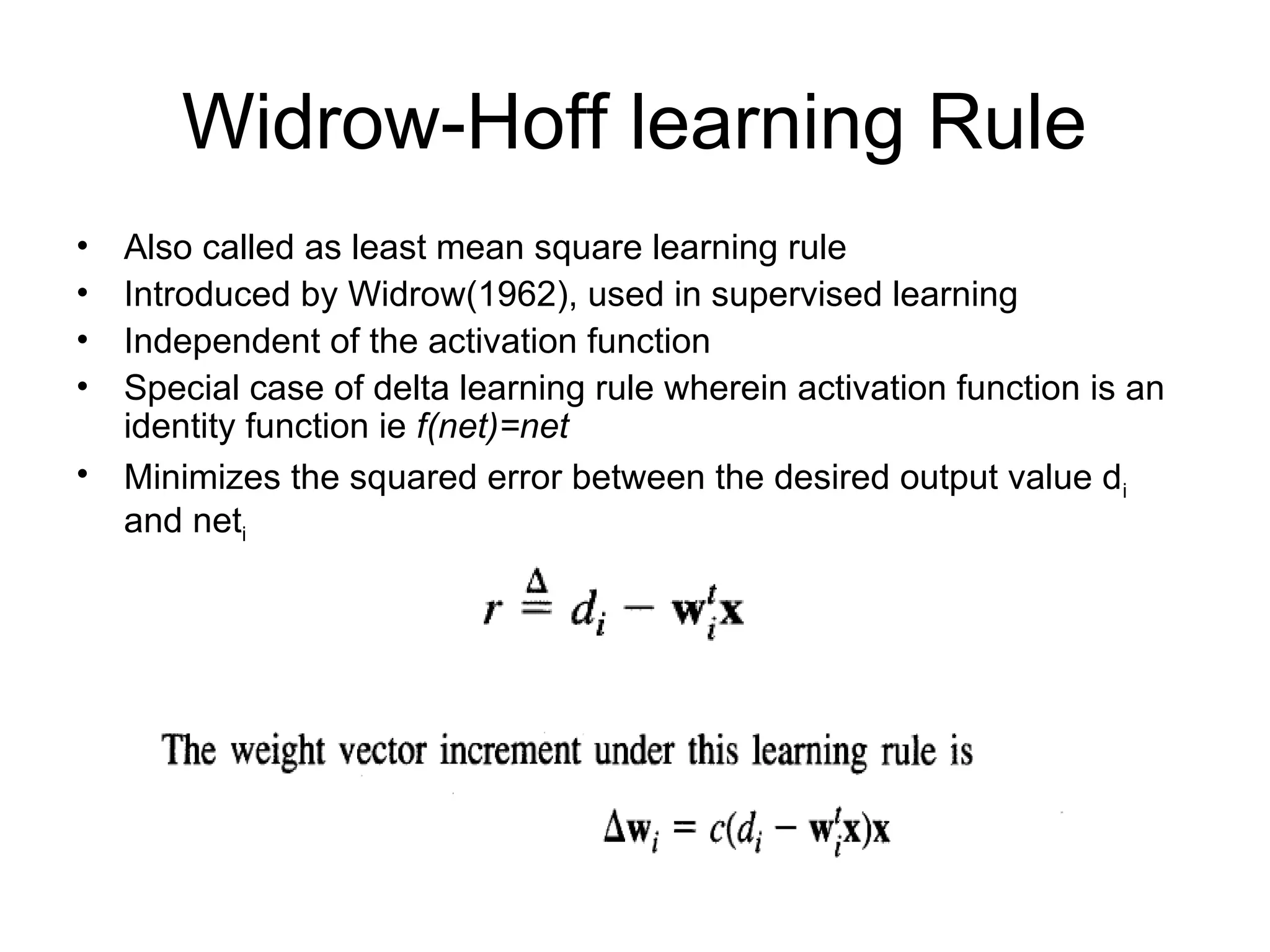
Widrow-Hoff learning Rule • Also called as least mean square learning rule • Introduced by Widrow(1962), used in supervised learning • Independent of the activation function • Special case of delta learning rule wherein activation function is an identity function ie f(net)=net • Minimizes the squared error between the desired output value di and neti

Winner-Take-All learning rules

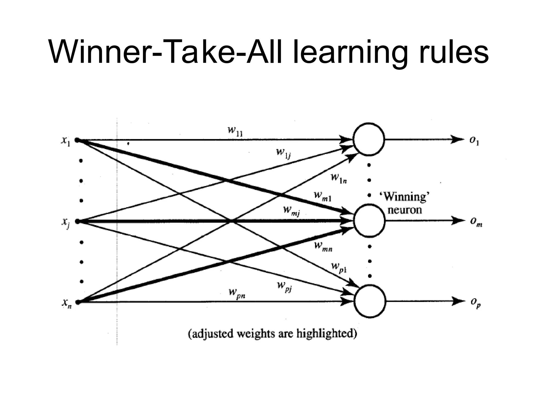
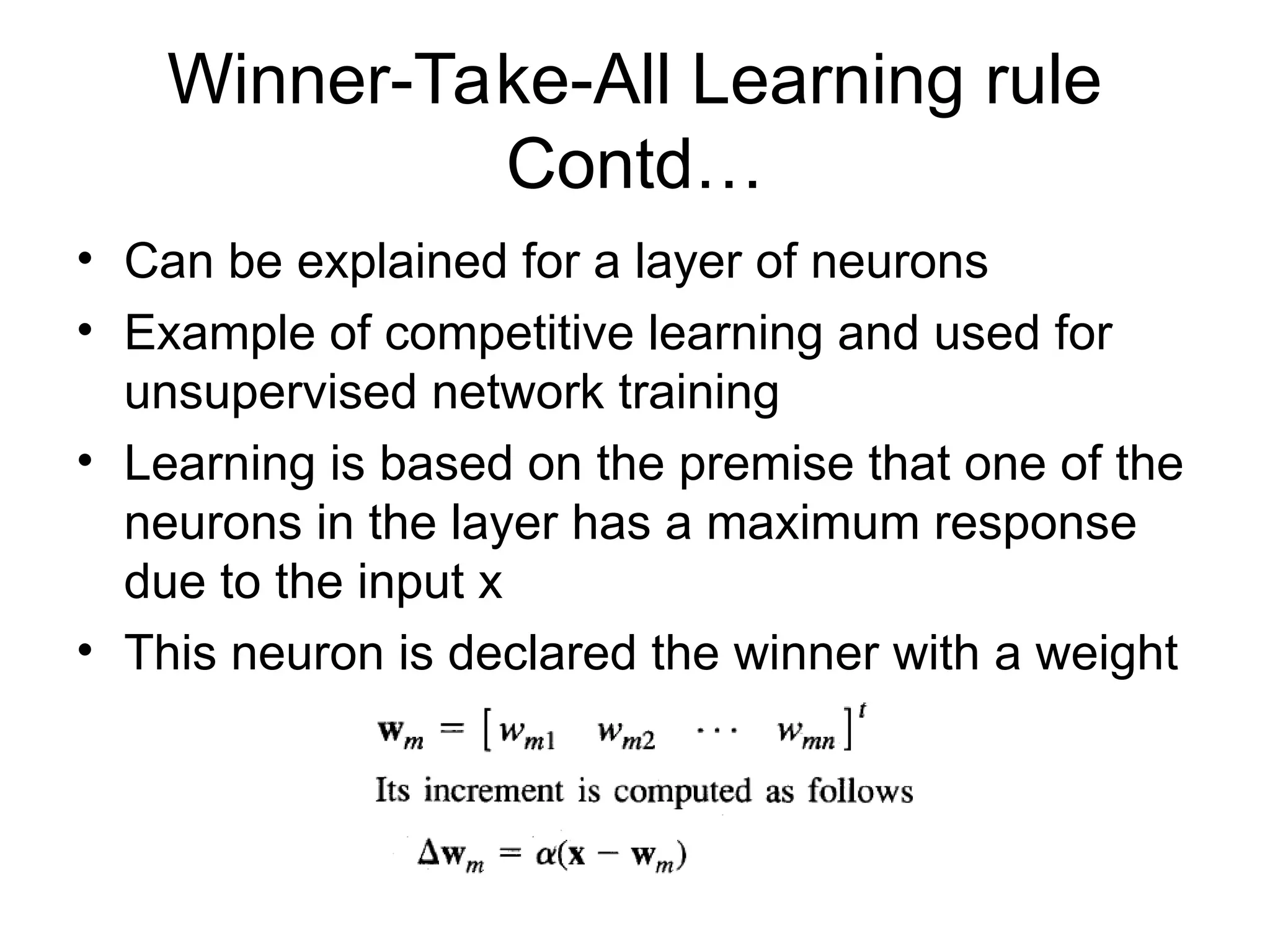
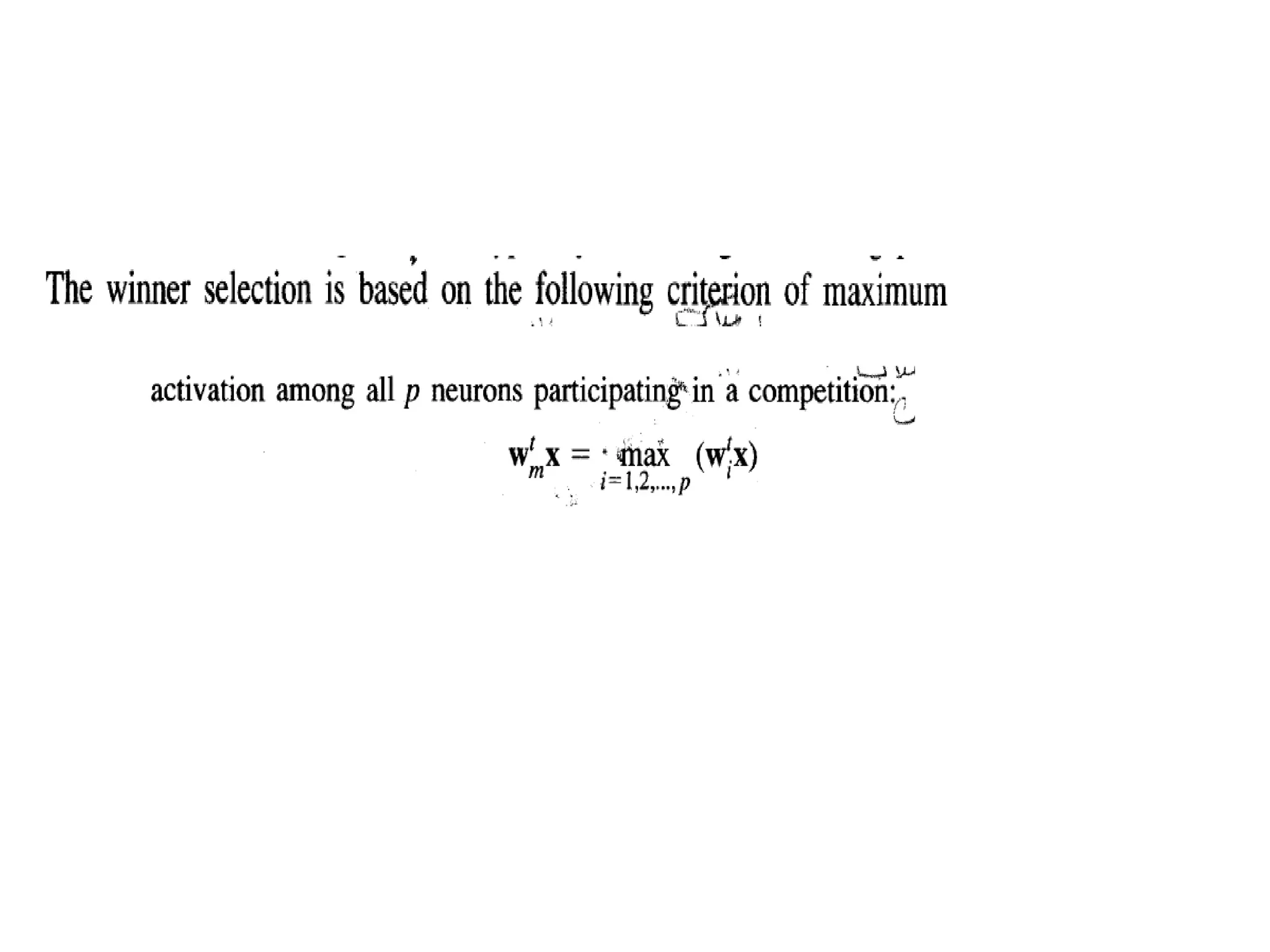
Winner-Take-All Learning rule Contd… • Can be explained for a layer of neurons • Example of competitive learning and used for unsupervised network training • Learning is based on the premise that one of the neurons in the layer has a maximum response due to the input x • This neuron is declared the winner with a weight

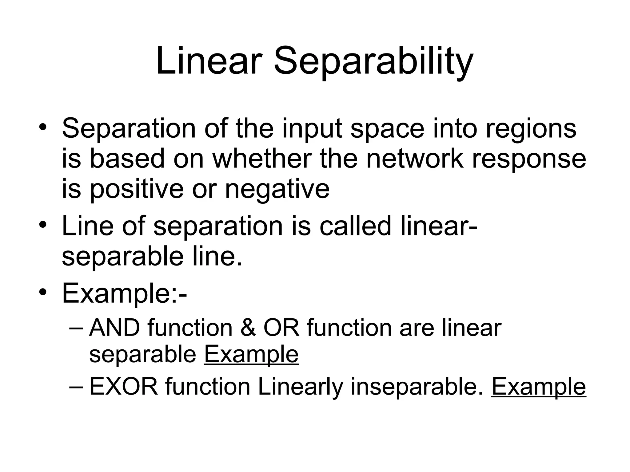
Linear Separability • Separation of the input space into regions is based on whether the network response is positive or negative • Line of separation is called linear- separable line. • Example:- – AND function & OR function are linear separable Example – EXOR function Linearly inseparable. Example

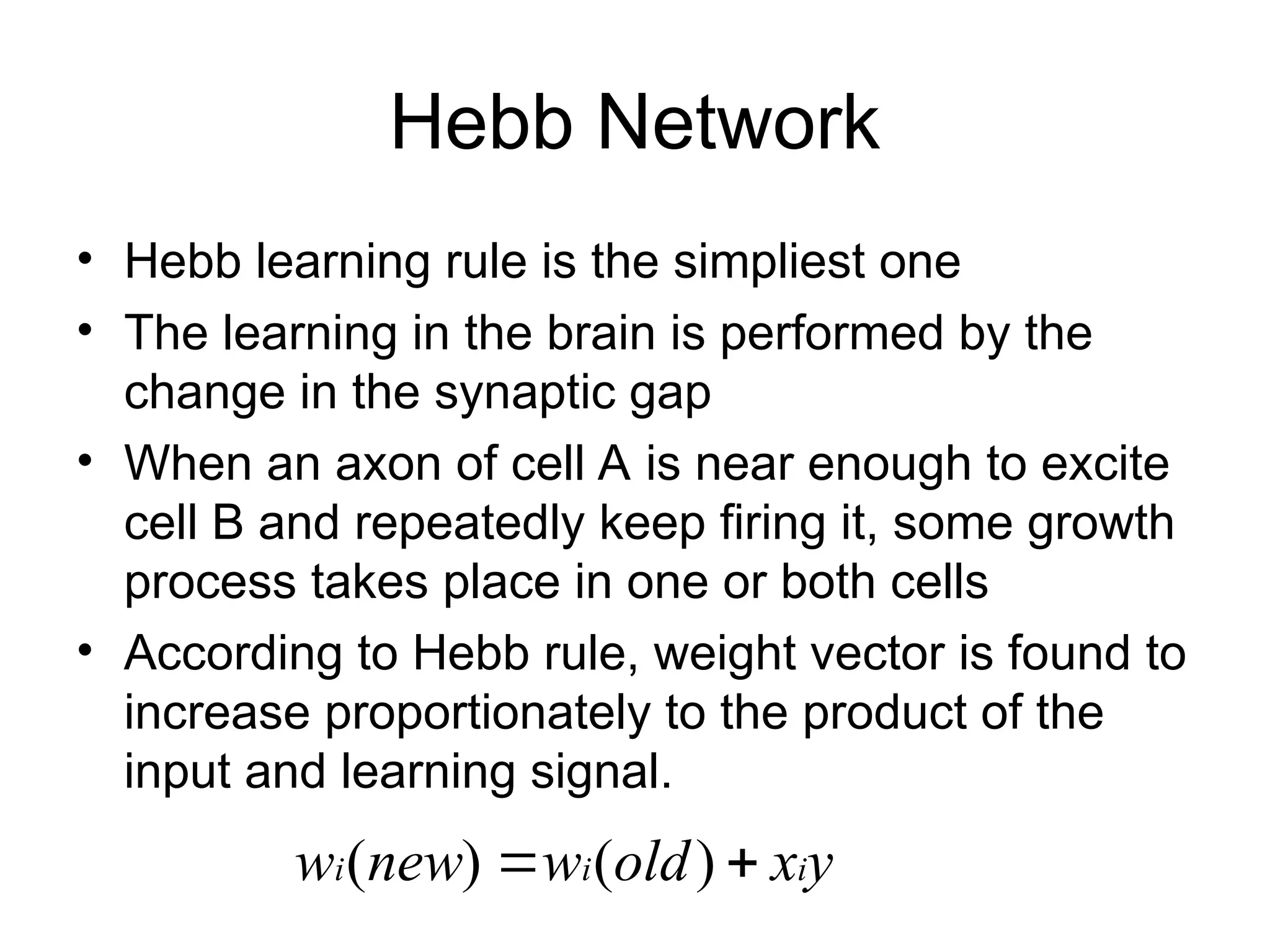
Hebb Network • Hebb learning rule is the simpliest one • The learning in the brain is performed by the change in the synaptic gap • When an axon of cell A is near enough to excite cell B and repeatedly keep firing it, some growth process takes place in one or both cells • According to Hebb rule, weight vector is found to increase proportionately to the product of the input and learning signal. y x old w new w i i i   ) ( ) (

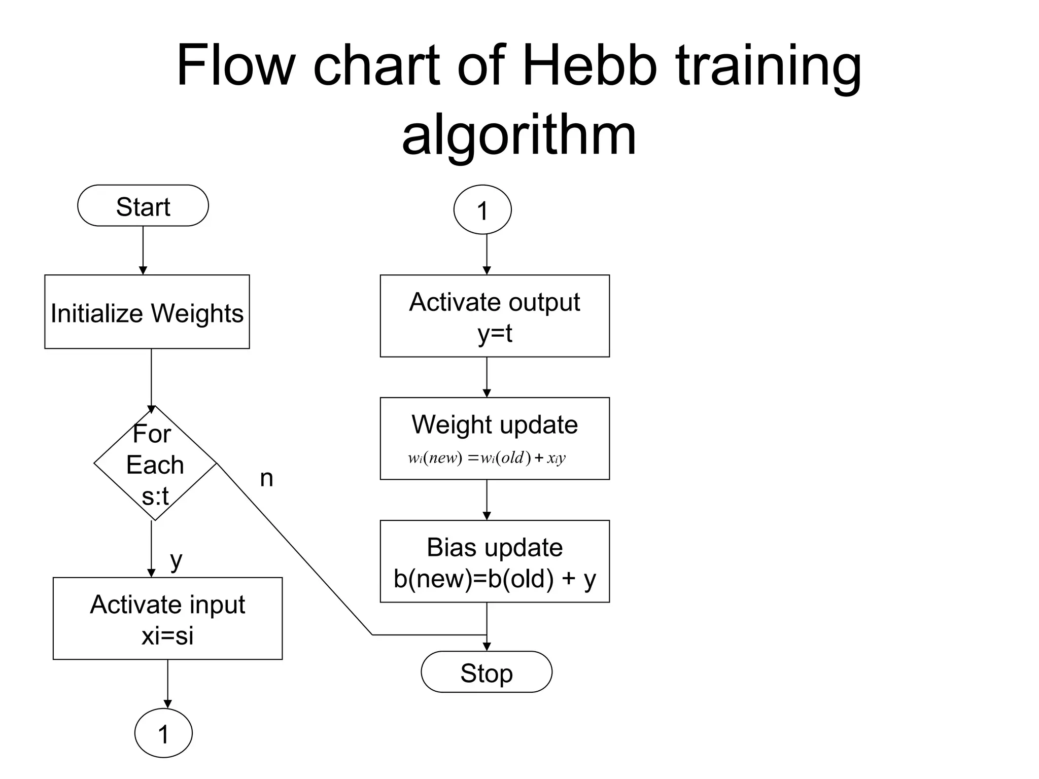
Flow chart of Hebb training algorithm Start Initialize Weights For Each s:t Activate input xi=si 1 1 Activate output y=t Weight update y x old w new w i i i   ) ( ) ( Bias update b(new)=b(old) + y Stop y n

• Hebb rule can be used for pattern association, pattern categorization, pattern classification and over a range of other areas • Problem to be solved: Design a Hebb net to implement OR function

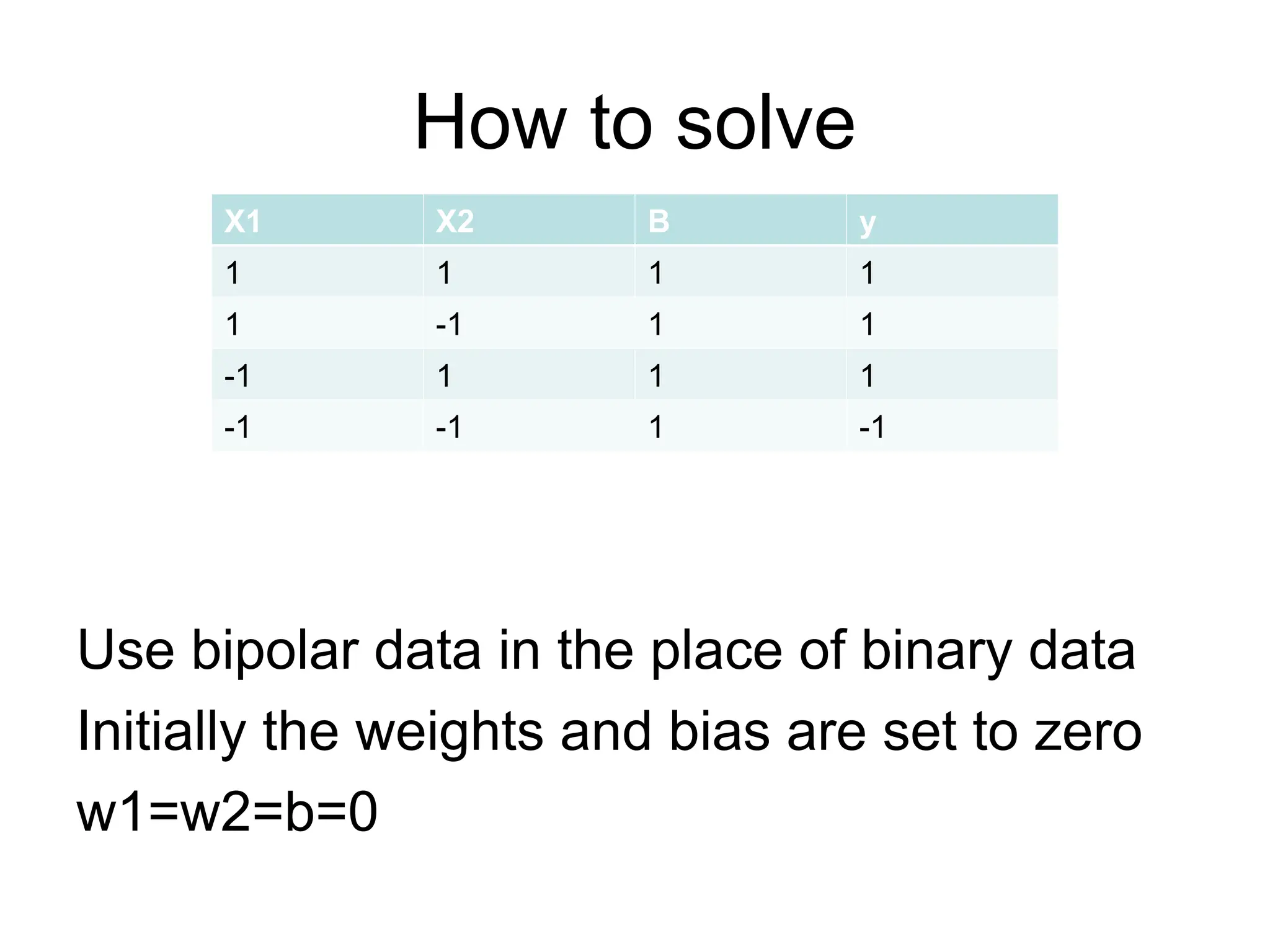
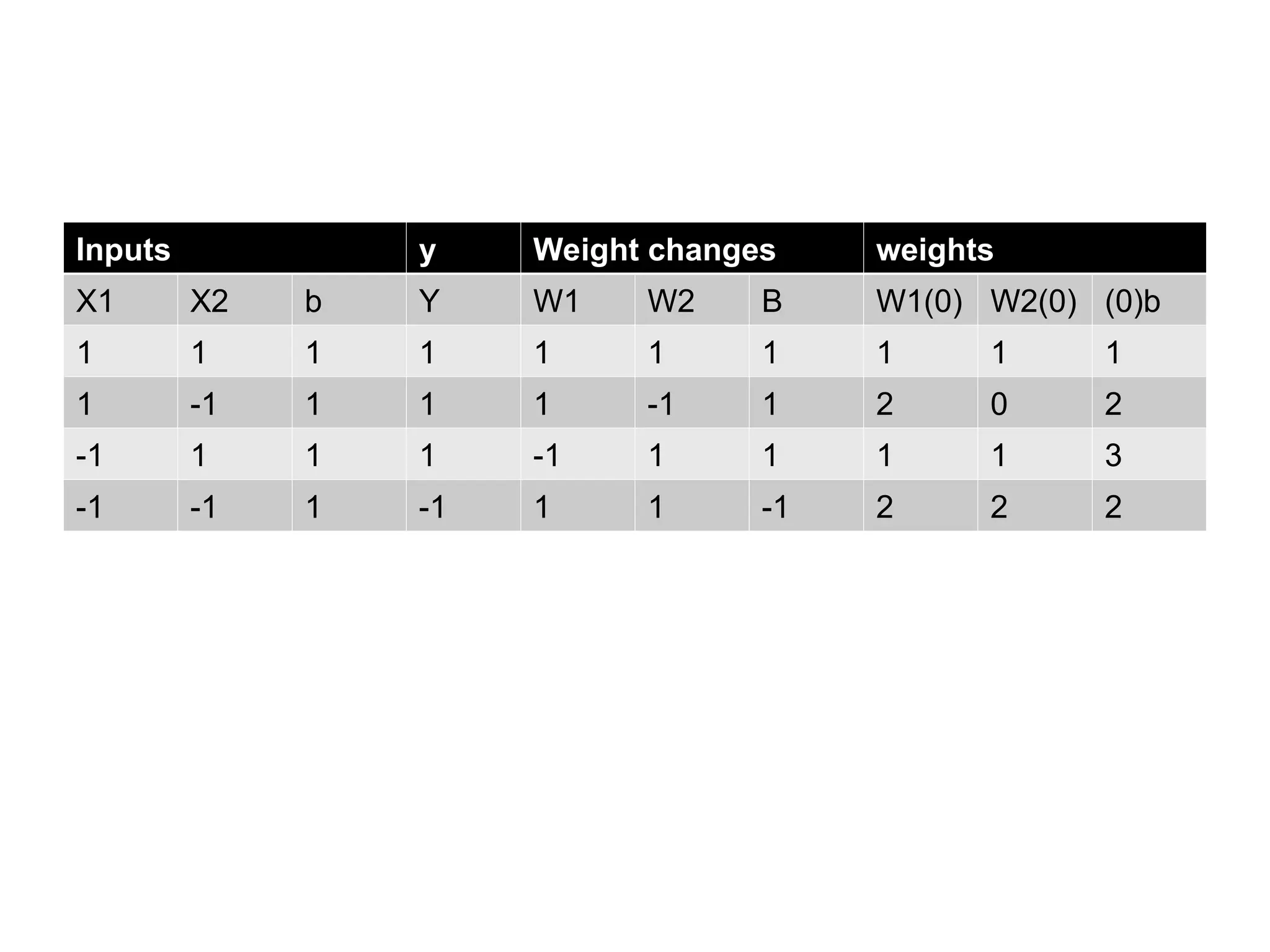
How to solve Use bipolar data in the place of binary data Initially the weights and bias are set to zero w1=w2=b=0 X1 X2 B y 1 1 1 1 1 -1 1 1 -1 1 1 1 -1 -1 1 -1

Inputs y Weight changes weights X1 X2 b Y W1 W2 B W1(0) W2(0) (0)b 1 1 1 1 1 1 1 1 1 1 1 -1 1 1 1 -1 1 2 0 2 -1 1 1 1 -1 1 1 1 1 3 -1 -1 1 -1 1 1 -1 2 2 2

Home work • Using the hebb rule, find the weights required to perform the following classification that given input patterns shown in figure

artificial-neural-networks overviewrev.ppt

More Related Content

Similar to artificial-neural-networks overviewrev.ppt

More from Pabitha Chidambaram

Recently uploaded

artificial-neural-networks overviewrev.ppt