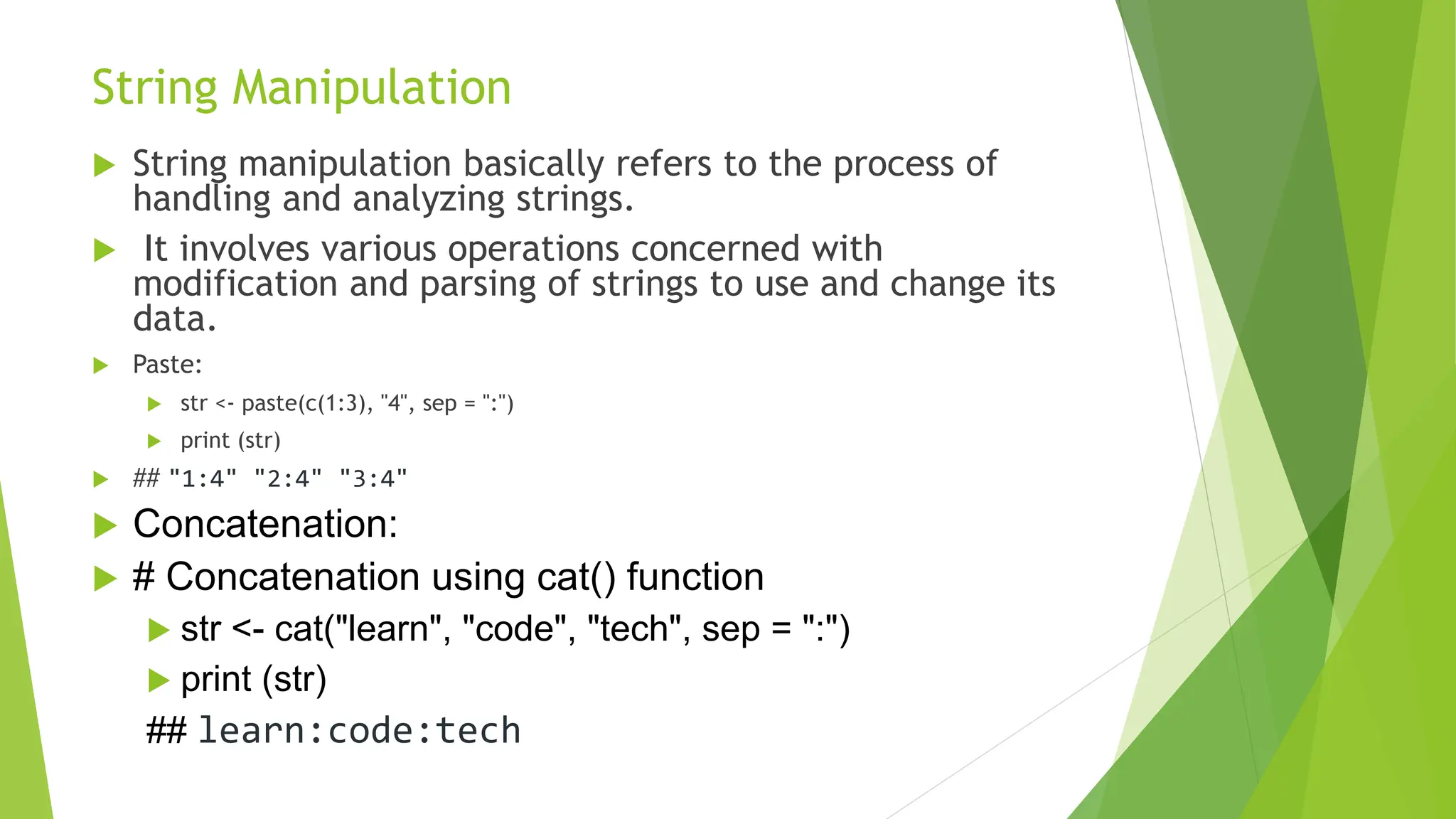
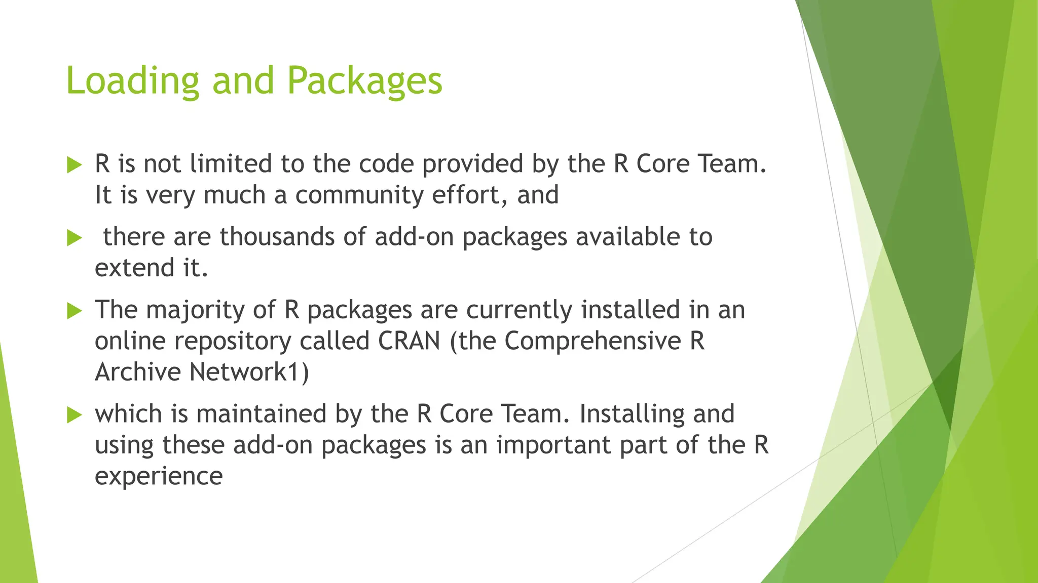
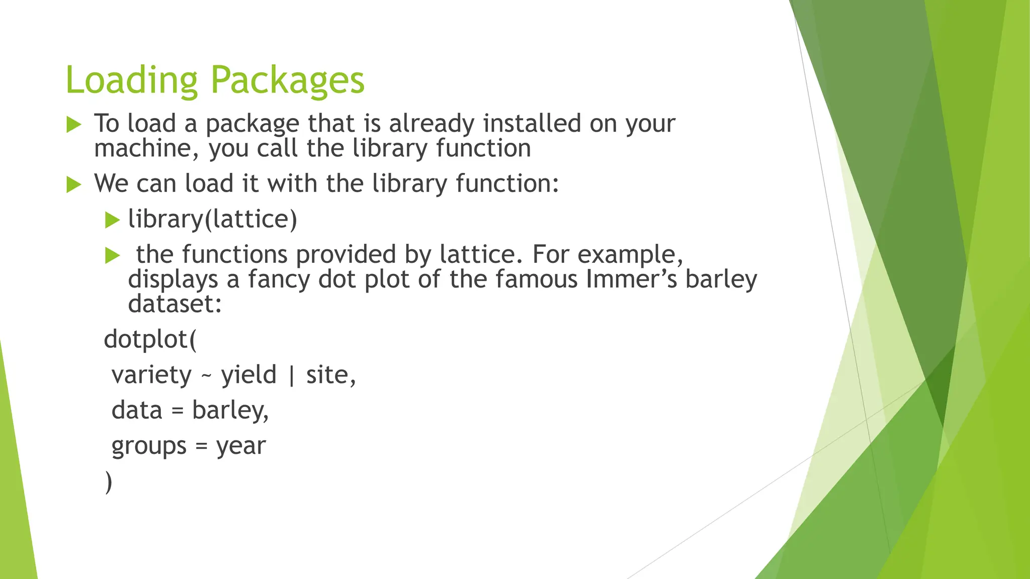
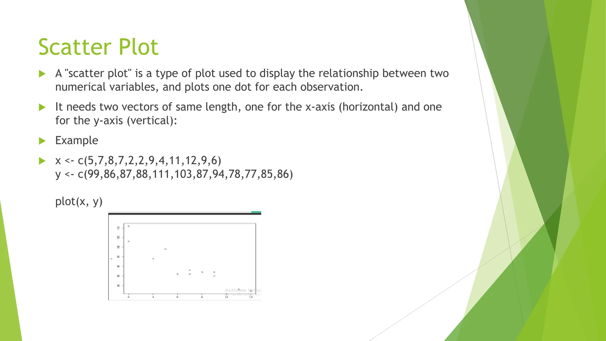
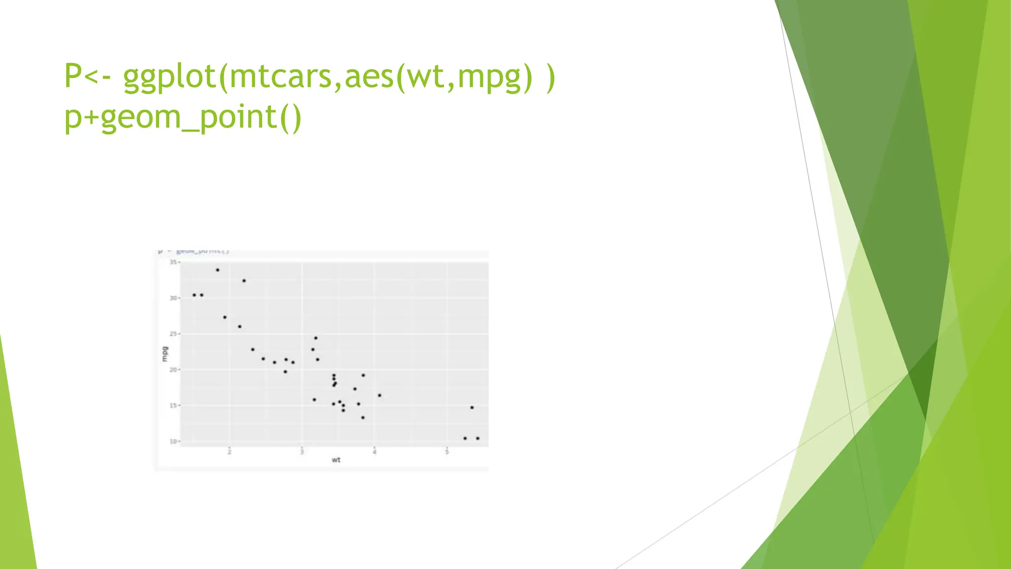
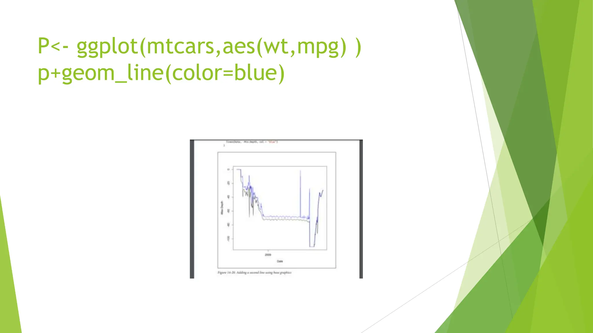
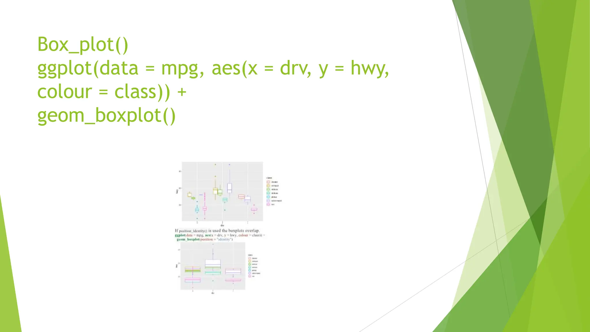
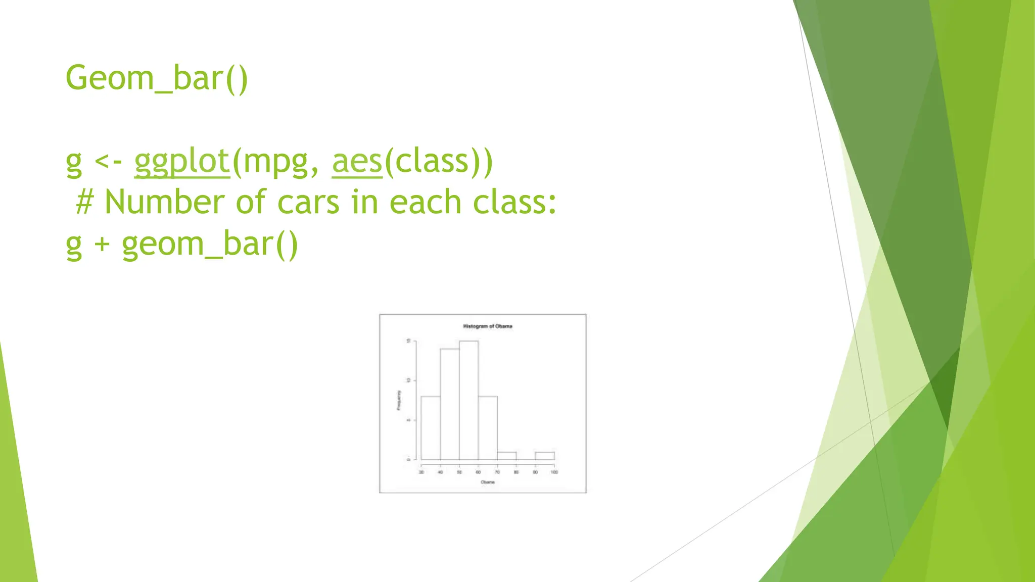
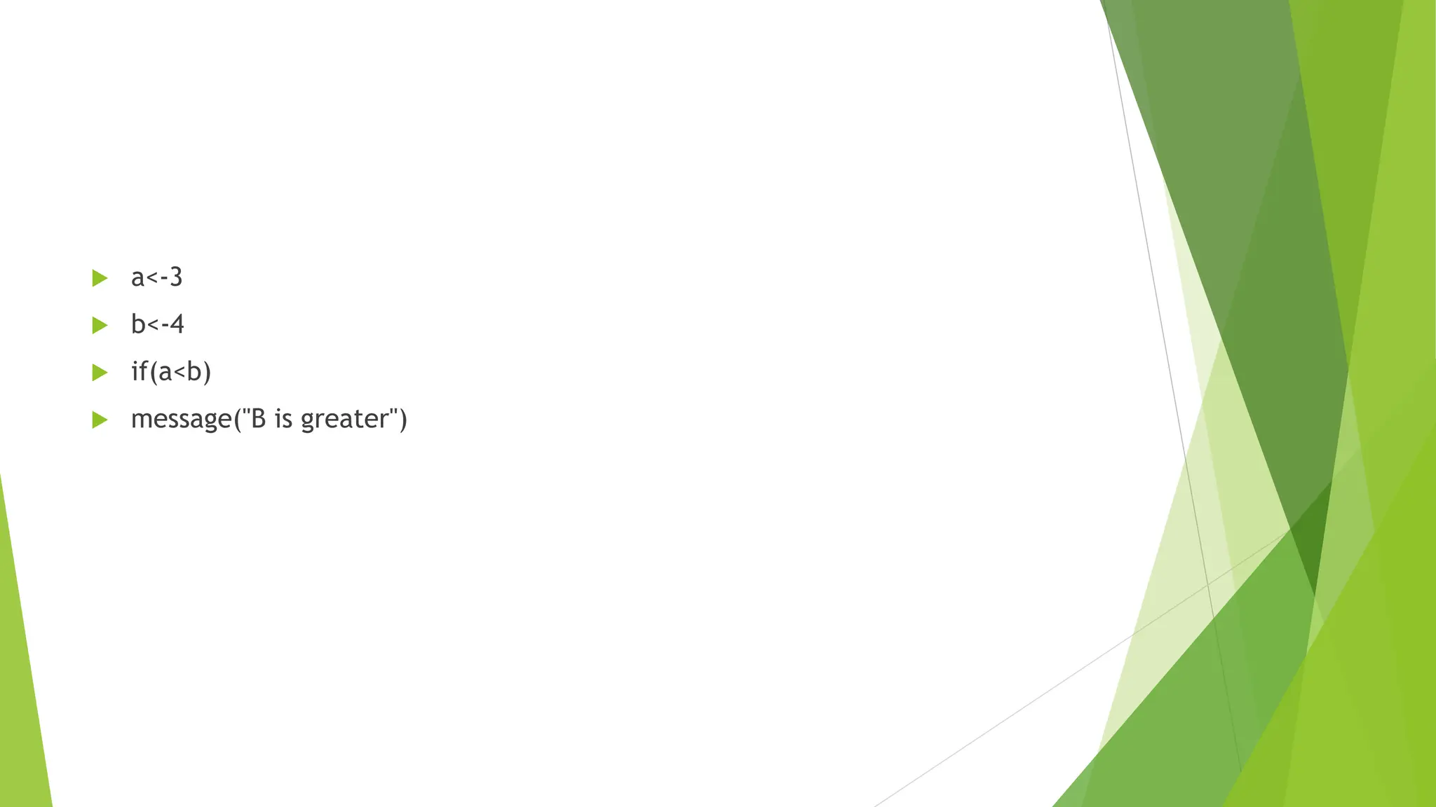
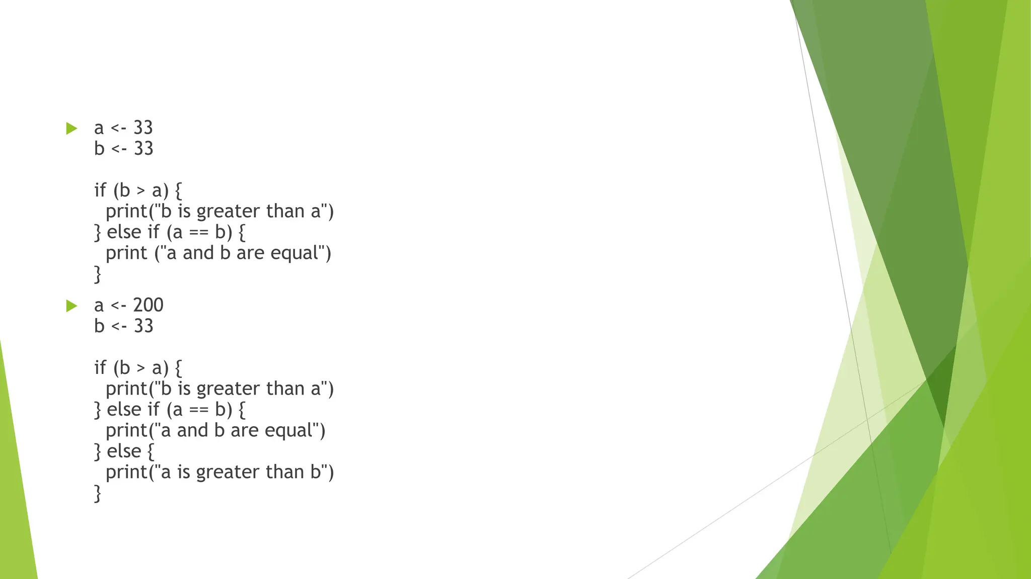
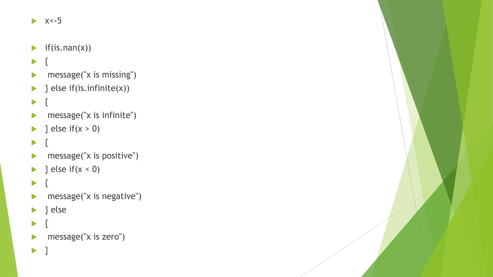
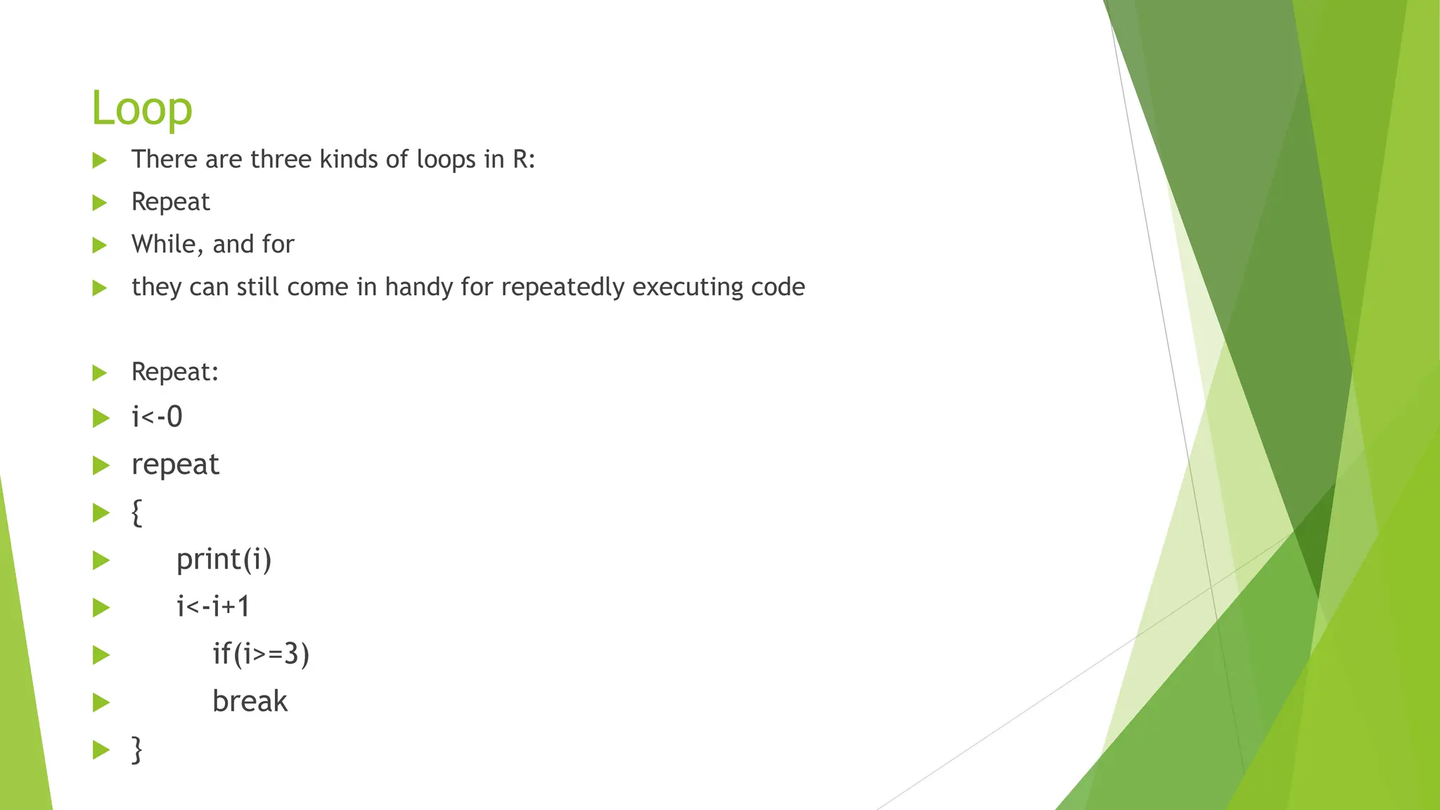
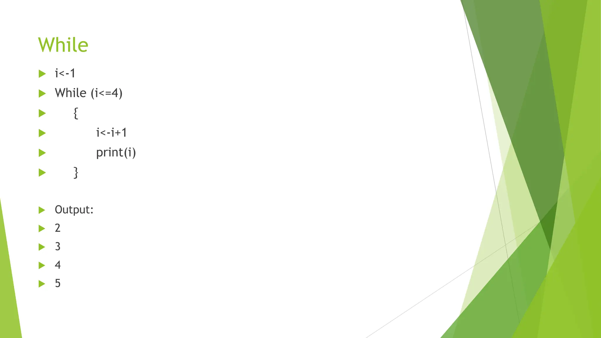
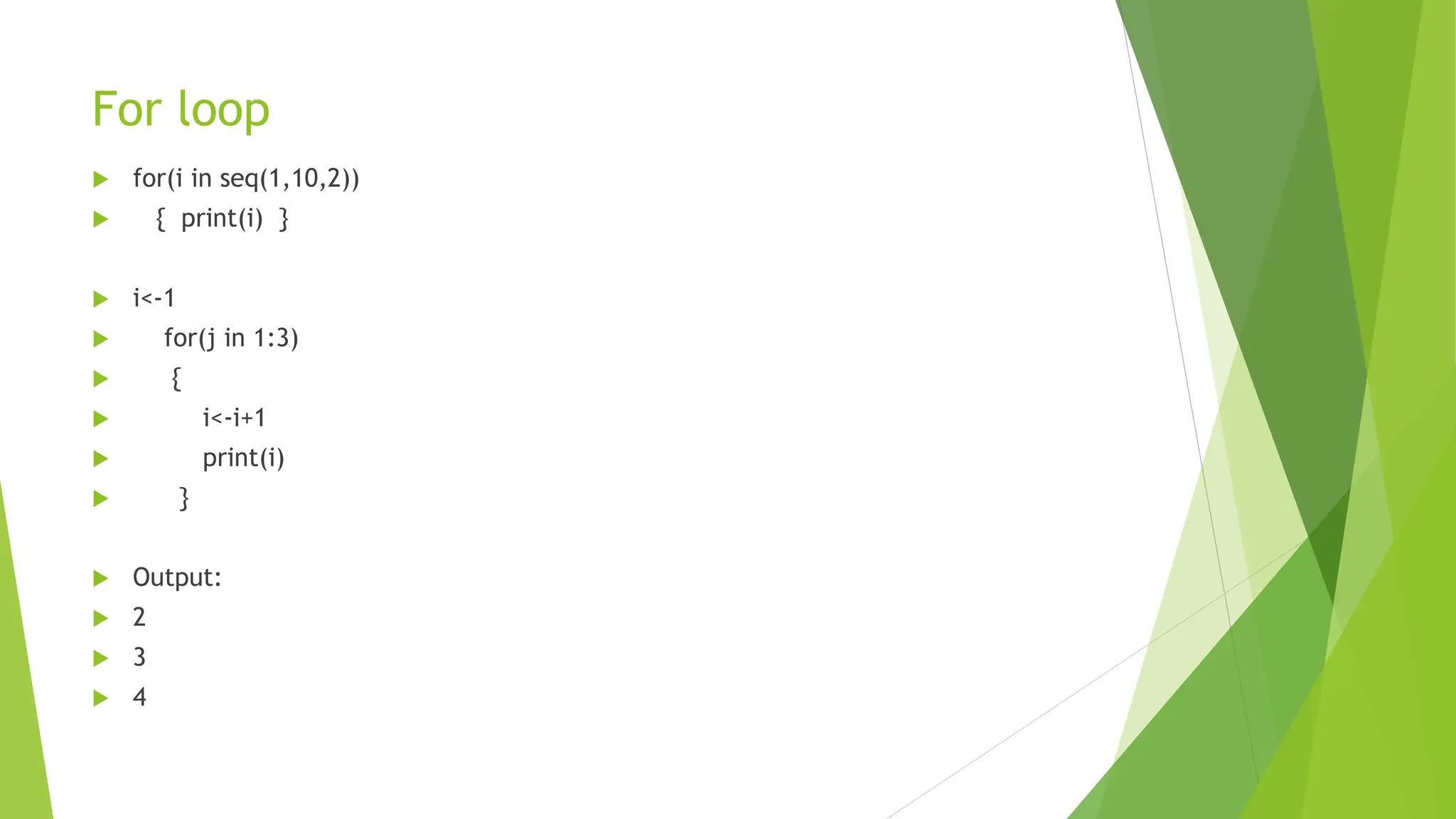
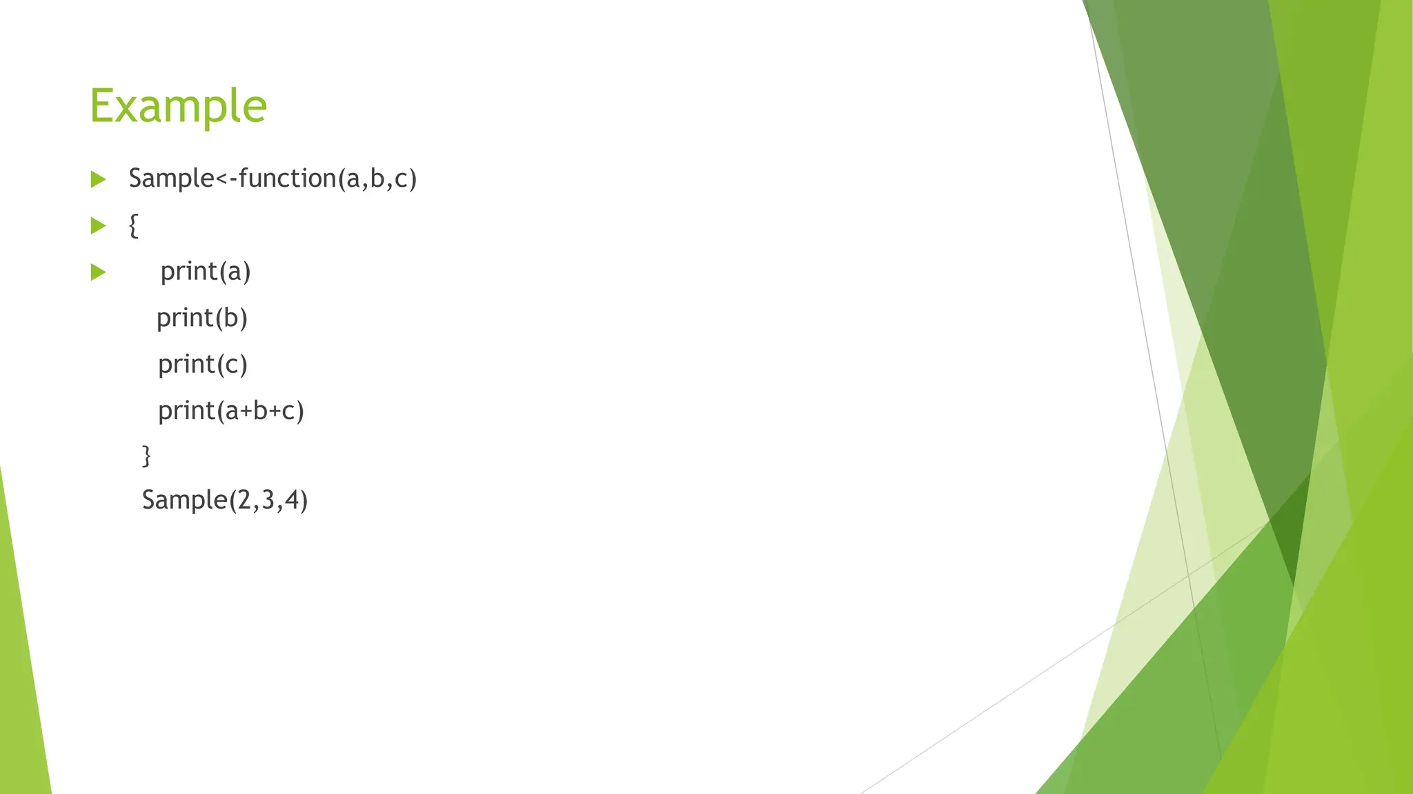
The document provides an overview of flow control, loops, functions, variable scope, string manipulation, and visualization in R programming. It details how to use conditional statements, different types of loops, and create functions, along with examples for each concept. Additionally, it discusses loading and using packages for data visualization, including scatter plots and bar graphs.

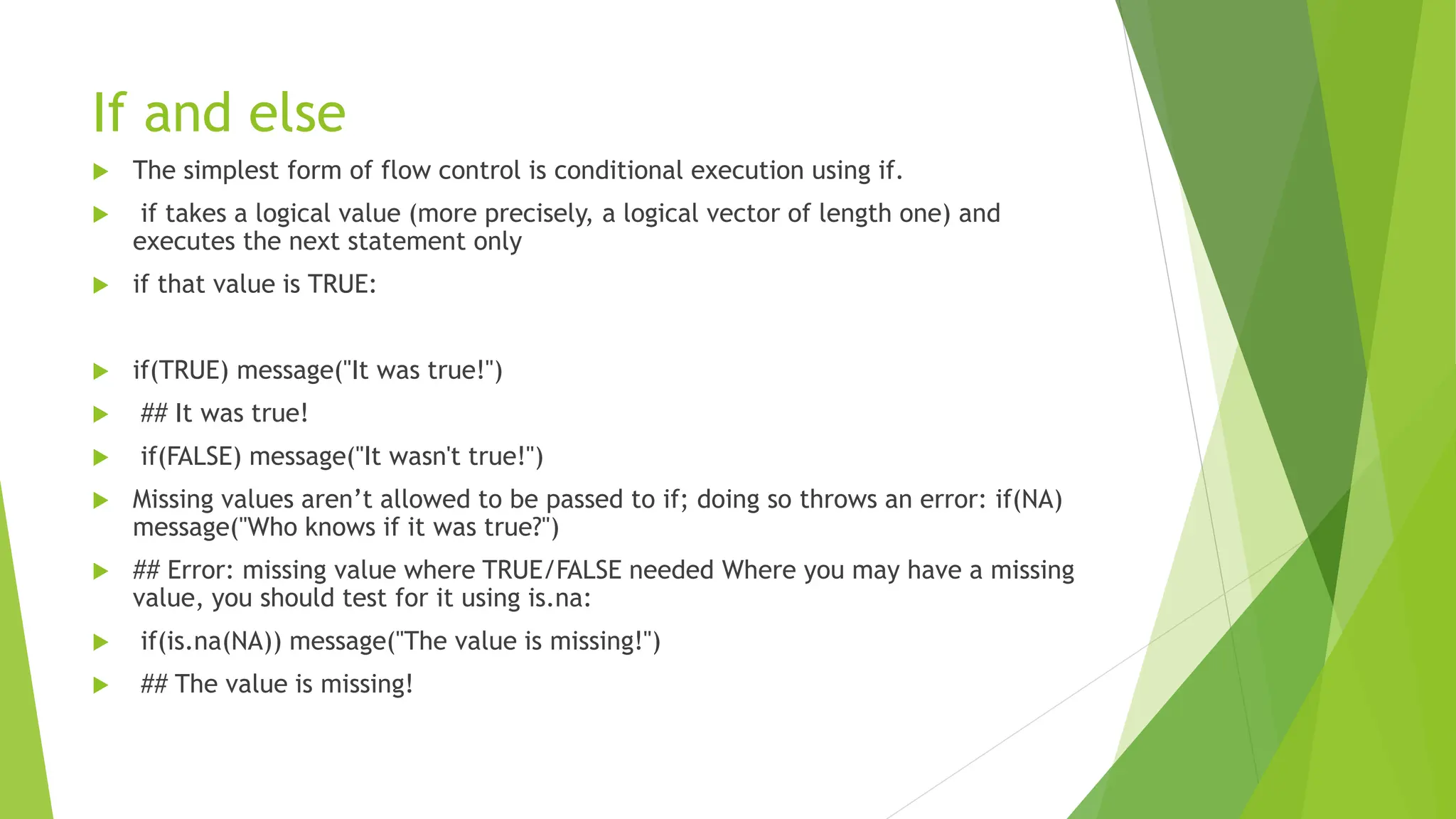
![ x <- 41 if (x > 10) { print("Above ten") if (x > 20) { print("and also above 20!") } else { print("but not above 20.") } } else { print("below 10.") } [1] "Above ten" [1] "and also above 20!"](https://image.slidesharecdn.com/flowcontrols-240614031857-d265ebfd-240614053125-88dbd434/75/app-app-app-ac99-net-7-2048.jpg)
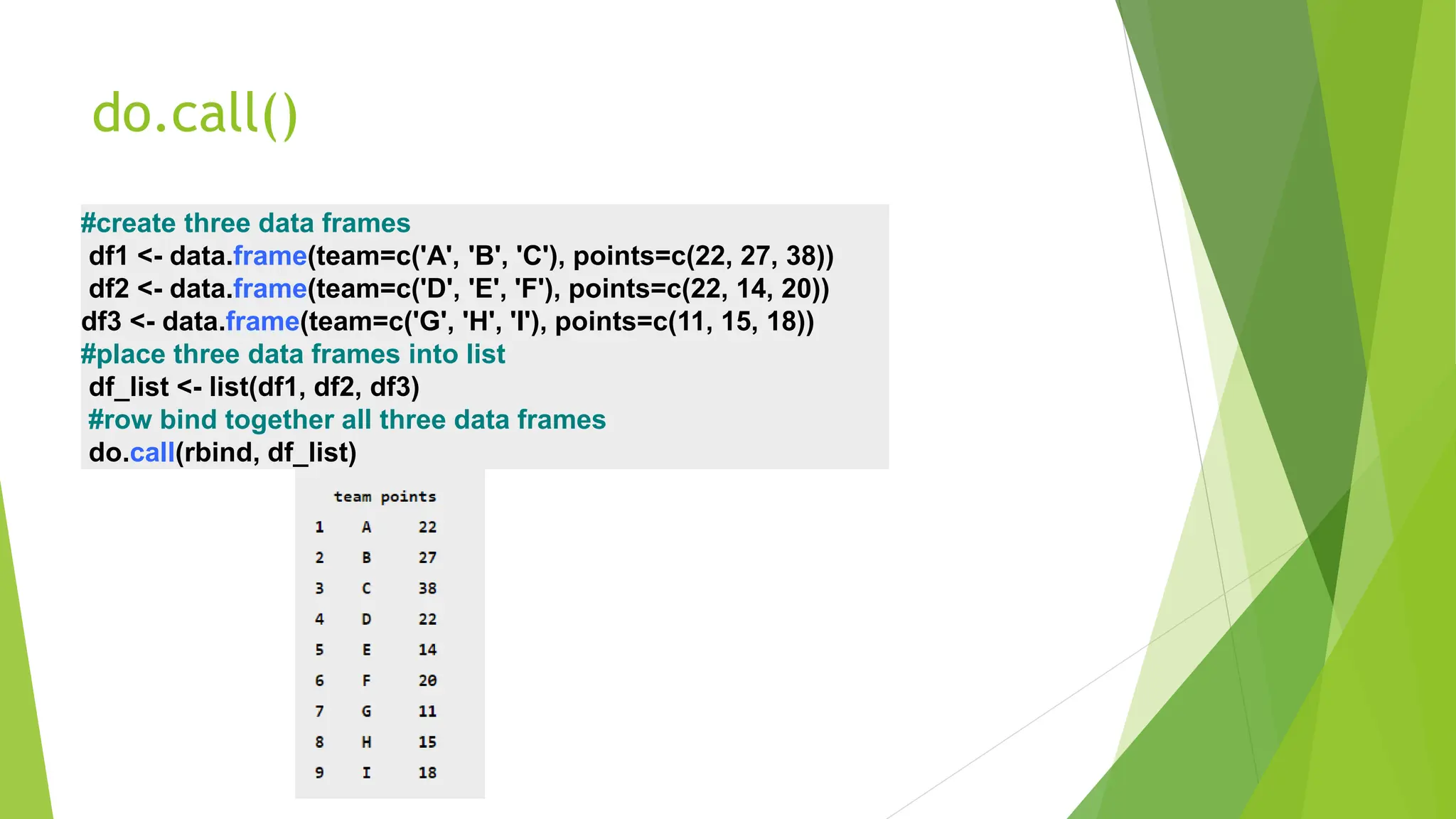
![Passing Functions to and from Other Functions Functions can be used just like other variable types, so we can pass them as arguments to other functions, and return them from functions. One common example of a function that takes another function as an argument is do.call. do.call(function(x, y) x + y, list(1:5, 5:1)) ## [1] 6 6 6 6 6](https://image.slidesharecdn.com/flowcontrols-240614031857-d265ebfd-240614053125-88dbd434/75/app-app-app-ac99-net-15-2048.jpg)
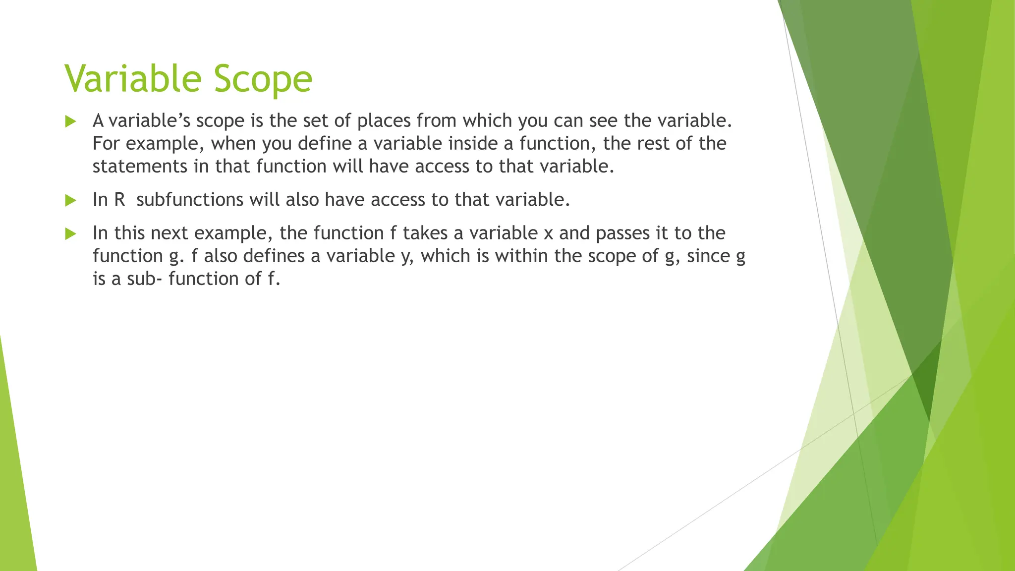
![ So, even though y isn’t defined inside g, the example works: f <- function(x) { y <- 1 g <- function(x) { (x + y) / 2 #y is used, but is not a formal argument of g } g(x) } f(sqrt(5)) #It works! y is magically found in the environment of f ## [1] 1.618](https://image.slidesharecdn.com/flowcontrols-240614031857-d265ebfd-240614053125-88dbd434/75/app-app-app-ac99-net-18-2048.jpg)