A modified backward/forward sweep-based method for reconfiguration of unbalanced distribution networks

A modified backward/forward sweep-based method for reconfiguration of unbalanced distribution networks

• 1.
  International Journal ofElectrical and Computer Engineering (IJECE) Vol. 9, No. 1, February 2019, pp. 85~101 ISSN: 2088-8708, DOI: 10.11591/ijece.v9i1.pp85-101  85 Journal homepage: http://iaescore.com/journals/index.php/IJECE A modified backward/forward sweep-based method for reconfiguration of unbalanced distribution networks Michell Quintero-Duran1 , John E. Candelo2 , Jose Soto-Ortiz3 1,2Applied Technologies Research Group, Universidad Nacional de Colombia, Sede Medellín, Colombia 2Department of Electrical Energy and Automation, Universidad Nacional de Colombia, Sede Medellín, Colombia 3Department of Electrical and Electronics Engineering, Universidad del Norte, Colombia Article Info ABSTRACT Article history: Received Feb 8, 2018 Revised Aug 17, 2018 Accepted Sep 18, 2018 A three-phase unbalanced power flow method can provide a more realistic scenario of how distribution networks operate. The backward/forward sweep- based power flow method (BF-PF) has been used for many years as an important computational tool to solve the power flow for unbalanced and radial power systems. However, some of the few available research tools produce many errors when they are used for network reconfiguration because the topology changes after multiple switch actions and the nodes are disorganized continually. This paper presents a modified BF-PF for three- phase unbalanced radial distribution networks that is capable of arranging the system topology when reconfiguration changes the branch connections. A binary search is used to determine the connections between nodes, allowing the algorithm to avoid those problems when reconfiguration is carried out, regardless of node numbers. Tests are made to verify the usefulness of the proposed algorithm in both the IEEE 13-node test feeder and the 123-node test feeder, converging in every run where constraints are accomplished. This approach can be used easily for a large-scale feeder network reconfiguration. The full version of this modified backward/forward sweep algorithm is available for research at MathWorks. Keywords: Adjacency matrix Backward/forward sweep-based method Binary search Power flow Radial Network Copyright © 2019 Institute of Advanced Engineering and Science. All rights reserved. Corresponding Author: Michell Quintero-Duran, Department of Electrical Energy and Automation Universidad Nacional de Colombia, Sede Medellín. Cra. 80 No. 65 - 223, Medellín, Antioquia, Colombia. Email: mjquinterod@unal.edu.co 1. INTRODUCTION Distribution networks are unbalanced systems in which loads are not precisely balanced through the network [1]–[3]. This feature rejects conventional balanced power flow methods, such as Newton–Raphson and Gauss–Seidel, to converge in order to find a solution for the non-linear power flow problem [4]–[6]. BF-PF has been used for several years to solve the radial power flow problem and is based on both the current and voltage Kirchhoff’s laws. This method was initially implemented for solving balanced radial distribution networks [7]. Nevertheless, the most commonly found distribution networks are unbalanced because most residential and commercial users use single or two-phase loads for home appliances and office equipment. On the other hand, most industrial users request three-phase feeders due to their load demands [8], [9]. Wang et al. presented an unbalanced BF-PF for real distribution systems [10], [11]. Diaz et al. developed a direct BF-PF for solving load power flows in AC droop-regulated microgrids [12]. Cun et al. performed a fuzzy approach to evaluate the power flow through the BF-PF method [13]. Kumar and Jain used the BF-PF algorithm for calculating both power losses and voltage regulation in radial systems with distributed generators and voltage regulators [14]. Nimal Madhu et al. incorporated a droop control to the DC
• 2.
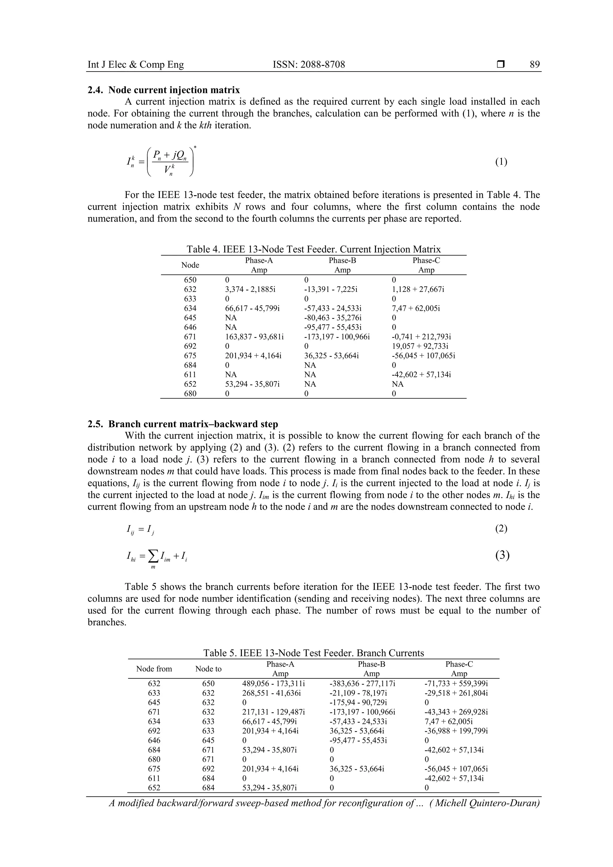
   ISSN: 2088-8708 IntJ Elec & Comp Eng, Vol. 9, No. 1, February 2019 : 85 - 101 86 equivalent power flow method for distribution and low voltage systems [15]. Xue et al. implemented an unbalanced three-phase distribution system power flow with distributed generation using the affine arithmetic self-validation method. An active distribution power flow analysis was performed using asymmetrical hybrid technique in [16]. Issicaba and Coelho proposed some improved methods inspired on the classical Cespedes’ load flow method, improving its efficiency in time response [17], [18]. Other authors have used the BF-PF for calculating load flow in distribution systems [19], [8], [9], [20]–[26]. With those improvements, BF-PF has become a useful tool for solving distribution network problems. Most of the approaches found in the literature and available for research for the power flow problem, consider a consecutive order in the node numeration. A downstream node should have always a higher number than its feeder bus. As an example, node number 2 is always fed by node number 1, never the contrary. This paper presents a modified backward/forward sweep-based power flow method for running the power flow of unbalanced radial networks that is suitable for the reconfiguration of distribution systems. The changes apply a binary search process to search the nodes, regardless of their numeration and organization. In that way, node number n could be fed by node number m. This approach allows researchers to make changes in the basic topology on any three-phase unbalanced radial distribution system. Considering the above, a feeder network reconfiguration process can be achieved even if the node numeration is not identified by a strict ascendant order. The rest of the document is organized as follows. Section 2 presents a brief explanation concerning the standard BF-PF method and its implementation on IEEE 13-node test feeder. Section 3 explains improvements developed in this paper, considering the binary search process for identifying the topology of the system. Section 4 presents the modified IEEE 13-node test feeder and the IEEE 123-node test feeder to make a reconfiguration. The evaluations in Section 5 provide results and discussion that guarantee the proficiency and usefulness of the proposed method. Finally, some conclusions are presented in Section 6. 2. STANDARD BF-PF The BF-PF is derived from both the voltage and current Kirchhoff’s laws [27], [28]. In Figure 1, we present a flowchart with the explanation of the steps of a standard BF-PF, which is commonly used for solving the power flow problem. We have divided this flowchart into three main sections: the input values, the process, and the output values of the algorithm. The inputs are given according to the distribution network test case and, for this test, we considered a total of seven inputs. The first input data correspond to the line segment, which provides information about the connections between the nodes of the radial distribution network. The second input is the voltage matrix that contains the voltage magnitudes and angles per phase at each node. The third input is a load matrix that contains information of the real and reactive power loads at each node. The fourth and fifth inputs are the identification of the main feeder as the slack node and the sources with voltage regulation as the PV nodes to maintain the voltage magnitude at each iteration. The sixth input is the impedance configuration matrix, given by the distribution network test case of study as a three-phase impedance matrix per branch for calculating voltage drop across the system. Finally, the seventh input is the mismatch limit that defines the stopping criterion, and we considered for this test a value of 1x10−4 . The process section concerns all calculations required to obtain a solution of the power flow and, thus, the power losses of the system. We have divided the process into six steps: topology of the system, current injection calculation, branch current calculation (backward step), node voltage updating (forward step), maximum voltage deviation calculation, convergence verification, and calculation of power losses. There are some temporary data saved for further calculations including: the current node injection matrix; branch current matrix; updated voltage matrix (i.e., the same initial voltage matrix but updated with the branch currents calculated); and maximum voltage deviation, which is the higher difference between voltages in the last and current iterations. To obtain convergence, this value must be lower or equal to the mismatch limit. We divided the output section into three groups. The first group corresponds to the branch currents, the second group is the node voltage magnitudes and angles, and the final group is the real power loss. In the following subsections, we explained how BF-PF works for solving the power flow problem in radial distribution networks. As an example, the IEEE 13-node test feeder has been selected to develop the complete process.
• 3.
  Int J Elec& Comp Eng ISSN: 2088-8708  A modified backward/forward sweep-based method for reconfiguration of ... ( Michell Quintero-Duran) 87 Figure 1. Flowchart for the standard BF-PF 2.1. Line segment matrix First, the algorithm requires the topology of the system. Thus, a line segment matrix is needed to verify the node connections. Table 1 presents the IEEE 13-node test feeder line matrix that can be accessed in [29], [30]. In that matrix, columns 1 and 2 are referred to as sending and receiving nodes of a branch, respectively. Column 3 introduces the length of branches. Finally, column 4 specifies the impedance configuration code, which provides information about the impedance matrix of each branch. Those configurations can be found in [29] and [30]. In addition, the number of rows must be exactly the number of branches that are in the system. The improvements proposed in this present paper are precisely in obtaining the current topology of the system considering a given line segment matrix. Those improvements are documented in Section 3.
• 4.
   ISSN: 2088-8708 IntJ Elec & Comp Eng, Vol. 9, No. 1, February 2019 : 85 - 101 88 Table 1. IEEE 13-Node Test Feeder. Line Segment Data From To Length (ft.) Configuration 632 645 500 603 632 633 500 602 633 634 0 XFM-1 645 646 300 603 650 632 2000 601 684 652 800 607 632 671 2000 601 671 684 300 604 671 680 1000 601 671 692 0 Switch 684 611 300 605 692 675 500 606 2.2. Initial voltage matrix Initial voltages are presented in a matrix that considers the number of phases of each node. Initially, this matrix will contain nominal line-neutral voltages represented in real or per unit values before the iteration process, and updating data at each iteration. The matrix has N rows, which represent the total number of nodes, and four columns, which represent the line-neutral voltage per phase at each node. The node numeration is in column 1 and line-neutral voltages for phases a, b, and c are in columns 2, 3, and 4, respectively. Whether a phase is not connected the initials NA (Non-Aplicable) appears. Table 2 presents the voltage matrix for the IEEE 13-node test feeder. Whether a regulator is found, the downstream node would have the same voltage that was set in the regulator. Table 2. IEEE 13-Node Test Feeder. Initial Voltage Matrix Node Phase-A (kV) Phase-B (kV) Phase-C (kV) 650 2,402 + 0i -1,201 – 2,08i -1,201 + 2,08i 632 2,45 – 0,1070i -1,316 – 2,129i -1,141 + 2,161i 633 2,402 + 0i -1,201 – 2,08i -1,201 + 2,08i 634 2,402 + 0i -1,201 – 2,08i -1,201 + 2,08i 645 NA -1,201 – 2,08i -1,201 + 2,08i 646 NA -1,201 – 2,08i -1,201 + 2,08i 671 2,402 + 0i -1,201 – 2,08i -1,201 + 2,08i 692 2,402 + 0i -1,201 – 2,08i -1,201 + 2,08i 675 2,402 + 0i -1,201 – 2,08i -1,201 + 2,08i 684 2,402 + 0i NA -1,201 + 2,08i 611 NA NA -1,2+ 2,08i 652 2,402 + 0i NA NA 680 2,402 + 0i -1,201 – 2,08i -1,201 + 2,08i 2.3. Load matrix A load matrix represents the power loads installed at each node per phase and it is required for further calculations. This matrix must have seven columns and N rows. The first column has the node numeration while columns 2–7 contain information concerning the active and reactive load on each node. They are organized in pairs per phase; for example, active and reactive load for phase a are in columns 2 and 3, respectively, and so on for phases b and c. Table 3 can be checked in [30]. Negative numbers represent a reactive power injection from capacitors installed in the node. Table 3. IEEE 13-Node Test Feeder. Load Matrix Node Phase-A (kW) Phase-A (kVAR) Phase-B (kW) Phase-B (kVAR) Phase-C (kW) Phase-C (kVAR) 650 0 0 0 0 0 0 632 8,5 5 33 19 58,5 34 633 0 0 0 0 0 0 634 160 110 120 90 120 90 645 0 0 170 125 0 0 646 0 0 230 132 0 0 671 393,5 225 418 239 443,5 254 692 0 0 0 0 170 151 675 485 -10 68 -140 290 12 684 0 0 0 0 0 0 611 0 0 0 0 170 -20 652 128 86 0 0 0 0 680 0 0 0 0 0 0
• 5.
  Int J Elec& Comp Eng ISSN: 2088-8708  A modified backward/forward sweep-based method for reconfiguration of ... ( Michell Quintero-Duran) 89 2.4. Node current injection matrix A current injection matrix is defined as the required current by each single load installed in each node. For obtaining the current through the branches, calculation can be performed with (1), where n is the node numeration and k the kth iteration. * k n n n k n P jQ I V        (1) For the IEEE 13-node test feeder, the matrix obtained before iterations is presented in Table 4. The current injection matrix exhibits N rows and four columns, where the first column contains the node numeration, and from the second to the fourth columns the currents per phase are reported. Table 4. IEEE 13-Node Test Feeder. Current Injection Matrix Node Phase-A Phase-B Phase-C Amp Amp Amp 650 0 0 0 632 3,374 - 2,1885i -13,391 - 7,225i 1,128 + 27,667i 633 0 0 0 634 66,617 - 45,799i -57,433 - 24,533i 7,47 + 62,005i 645 NA -80,463 - 35,276i 0 646 NA -95,477 - 55,453i 0 671 163,837 - 93,681i -173,197 - 100,966i -0,741 + 212,793i 692 0 0 19,057 + 92,733i 675 201,934 + 4,164i 36,325 - 53,664i -56,045 + 107,065i 684 0 NA 0 611 NA NA -42,602 + 57,134i 652 53,294 - 35,807i NA NA 680 0 0 0 2.5. Branch current matrix–backward step With the current injection matrix, it is possible to know the current flowing for each branch of the distribution network by applying (2) and (3). (2) refers to the current flowing in a branch connected from node i to a load node j. (3) refers to the current flowing in a branch connected from node h to several downstream nodes m that could have loads. This process is made from final nodes back to the feeder. In these equations, Iij is the current flowing from node i to node j. Ii is the current injected to the load at node i. Ij is the current injected to the load at node j. Iim is the current flowing from node i to the other nodes m. Ihi is the current flowing from an upstream node h to the node i and m are the nodes downstream connected to node i. ij jI I (2) hi im i m I I I  (3) Table 5 shows the branch currents before iteration for the IEEE 13-node test feeder. The first two columns are used for node number identification (sending and receiving nodes). The next three columns are used for the current flowing through each phase. The number of rows must be equal to the number of branches. Table 5. IEEE 13-Node Test Feeder. Branch Currents Node from Node to Phase-A Phase-B Phase-C Amp Amp Amp 632 650 489,056 - 173,311i -383,636 - 277,117i -71,733 + 559,399i 633 632 268,551 - 41,636i -21,109 - 78,197i -29,518 + 261,804i 645 632 0 -175,94 - 90,729i 0 671 632 217,131 - 129,487i -173,197 - 100,966i -43,343 + 269,928i 634 633 66,617 - 45,799i -57,433 - 24,533i 7,47 + 62,005i 692 633 201,934 + 4,164i 36,325 - 53,664i -36,988 + 199,799i 646 645 0 -95,477 - 55,453i 0 684 671 53,294 - 35,807i 0 -42,602 + 57,134i 680 671 0 0 0 675 692 201,934 + 4,164i 36,325 - 53,664i -56,045 + 107,065i 611 684 0 0 -42,602 + 57,134i 652 684 53,294 - 35,807i 0 0
• 6.
   ISSN: 2088-8708 IntJ Elec & Comp Eng, Vol. 9, No. 1, February 2019 : 85 - 101 90 2.6. Node voltage matrix–forward step With the forward step, it is possible to update the voltages in each node of the system. This matrix allows identifying the voltage profile while the branch currents are updated in the previous step as the voltage drop depends on the branch impedance and the current flowing on the branch. Node voltages are updated using both the configuration impedance matrix [29], [30] and the branch current matrix by using the general (4). PV nodes will have the same nominal value in all iterations, such node is the substation and all downstream nodes connected to a regulator. This process starts from the substation node toward the final nodes. j i ij ijV V Z I   (4) Equations (5)–(11) are the special conventions obtained from (4), considering that we can calculate the voltages for three-phase, two-phase, and single-phase branches. ja ia aa n ab n ac n ij a jb ib ba n bb n bc n ij b jc ic ca n cb n cc n ij c V V Z Z Z I V V Z Z Z I V V Z Z Z I                                               (5) ja ij aia aa n ab n jb ij bib ba n bb n V IV Z Z V IV Z Z                           (6) jb ij bib bb n bc n jc ij cic cb n cc n V IV Z Z V IV Z Z                           (7) ja ij aia aa n ac n jc ij cic ca n cc n V IV Z Z V IV Z Z                           (8) ja ia aa n ij aV V Z I    (9) jb ib bb n ij bV V Z I    (10) jc ic cc n ij cV V Z I    (11) The subscripts a, b, and c refer to the branches’ phases. The impedance matrix is a reduction found in all IEEE test case formats [29], [30]. This reduction is derived from the Carson equations, which can be consulted in [31]. Table 6 presents the node voltages updated in the first iteration concerning the IEEE 13-node test feeder. This matrix must have N rows and four columns. The first column is for node numeration while voltage per phase is registered in columns 2–4, considering phases a, b, and c. Table 6. IEEE 13-Node Test Feeder. Node Voltage Matrix Node Phase-A Phase-B Phase-C kV kV kV 650 2,402 + 0i -1,201 – 2,08i -1,201 + 2,08i 632 2,45 – 0,107i -1,316 – 2,129i -1,141 + 2,161i 633 2,436 – 0,134i -1,319 – 2,134i -1,117 + 2,136i 634 2,360 – 0,172i -1,312 – 2,068i -1,064 + 2,097i 645 NA -1,319 – 2,108i -1,142 + 2,169i 646 NA -1,321 – 2,102i -1,142 + 2,171i 671 2,408 – 0,144i -1,329 – 2,09i -1,068 + 2,147i 692 2,433 – 0,222i -1,325 – 2,186i -1,055 + 2,089i 675 2,418 – 0,232i -1,334 – 2,187i -1,053 + 2,085i 684 2,406 – 0,145i NA -1,064 + 2,146i 611 NA NA -1,056 + 2,145i 652 2,392 – 0,142i NA NA 680 2,408 – 0,144i -1,329 – 2,090i -1,068 + 2,147i
• 7.
  Int J Elec& Comp Eng ISSN: 2088-8708  A modified backward/forward sweep-based method for reconfiguration of ... ( Michell Quintero-Duran) 91 2.7. Convergence requirement The BF-PF has an iterative process and after each single iteration the node current injection, branch currents, and node voltages are updated until the convergence rate is fulfilled. The minimum allowed mismatch in the absolute subtraction between voltage magnitude of last and current iteration is 1 x 10−4 for each node. The error can be calculated at each iteration as shown in (12), where e is the mismatch and k is the current iteration.    1k k i iabs V abs V e   (12) 2.8. Real power loss calculation When convergence is reached, the total real power losses can be computed using (13), where l is the branch number, real(Zl) is the real part of the impedance matrix of the lth branch, and Il is the current flowing per branch l in each phase. 2 1 ( ) nbr loss l l l P real Z I    (13) One of the main problems of programming this method is that the BF-PF requires that the nodes are organized in an ascendant manner. That means that a node number 2 can be fed by a node number 1, otherwise the algorithm will show some errors. In the next section, we present a modified part of the algorithm to deal with different node number orders. 3. MODIFIED BF-PF In this section, we present a procedure applied to identify the topology and calculate branch currents and node voltages in a radial unbalanced distribution network, independent from the node number order. As in the standard BF-PF, the inputs considered in the algorithm are given by the feeder test case. The outputs are the same as those presented in Figure 1, namely, branch currents, nodes voltages, and active power losses. 3.1. Loading the case study The first step is to load the feeder test case that contains the slack node, the number of switches, and the data of lines, nodes, and regulators. The number of branches is expressed in (14) and can be used to verify that in case of multiple changes in the topology, the new network is radial, where nbr is the number of branches and N is the total number of nodes. 1nbr N  (14) 3.2. First radiality constraint verification In this step, we verify that the number of nodes is the same to that calculated in (14) when the data from the feeder test case is obtained. For example, in the IEEE 13-node test feeder, the number of nodes is N=13 and the number of branches is nbr=12. In this example, the algorithm must identify if a low number of branches is connected and, thus, the distribution network does not comply with radiality. 3.3. Neighborhood matrix The neighborhood matrix is defined as the identification of neighboring nodes [4]. This approach shows a list of connections between nodes with the rest of the system. As an example, the neighborhood matrix for the IEEE 13-node test feeder is presented in Table 7. It must contain two columns and two times nbr rows. Column 1 presents the node number and column 2 refers to all nodes connected to the node in column 1. If a node is connected to more than one other node, then it appears more than once in the first column. From Table 7, node 632 is connected to 650, 633, 645, and 671. 3.4. Determining the type of node Once the neighborhood matrix is built, a mf_mt matrix is necessary to identify the number of branches connected to each node. Table 8 presents the mf_mt matrix for the IEEE 13-node test feeder, which has N rows and four columns. The node number is in the first column. The starting row, where node n is found into the first column of the neighborhood matrix, is placed in column 2. The ending row, where the
• 8.
   ISSN: 2088-8708 IntJ Elec & Comp Eng, Vol. 9, No. 1, February 2019 : 85 - 101 92 node n is in the first column of the neighborhood matrix, is specified in column 3. Column 4 contains the subtraction between columns 3 and 2 [27]. Table 7. IEEE 13-Node Test Feeder. Neighboring Matrix Column 1–part 1 Column 2–part 1 Column 1–part 2 Column 2–part 2 Node Connected to Node Connected to 650 632 671 680 632 650 671 684 632 633 671 692 632 645 680 671 632 671 684 671 633 632 684 652 633 634 684 611 634 633 652 684 645 632 611 684 645 646 692 671 646 645 692 675 671 632 675 692 Table 8. IEEE 13-Node Test Feeder. Mf_mt Matrix Node number mf (initial row) mt (ending row) mt-mf 650 1 1 0 632 2 5 3 633 6 7 1 634 8 8 0 645 9 10 1 646 11 11 0 671 12 15 3 680 16 16 0 684 17 19 2 652 20 20 0 611 21 21 0 692 22 23 1 675 24 24 0 As shown in this table, the node 650 starts in the first row of the neighborhood matrix and ends in this same row, which indicates that it has only one connection through a branch to one other node (632). Moreover, node 632 starts in row 2 from the neighborhood matrix and ends in row 5, which indicates that this node is connected through four branches to four nodes. Column 4 presents the case when a node is an ending node, intermediate node, or a junction node. This is determined as follows [27]: 1. An ending node refers to the node that connects only to another node through one or more branches. For this case, the value in column 4 is zero. 2. An intermediate node can be identified as the node connected to two other nodes through one or more branches for each pair of nodes. For this case, the value in column 4 is 1. 3. A junction node is the element that is used to connect more than two nodes with more than two branches. For this case, the value in column 4 is greater than 1. The slack node must be found in the mf_mt matrix and identify its position, and not to be considered as an ending node. Because the slack node could have one or more connections, it must be considered as the root when searching the topology of the system. The binary search initializes from the slack node to find each connection to the rest of the nodes; therefore, we considered in this paper to explain how we deal with the topology to avoid mistakes when the connections change, and the search is needed to reconfigure. 3.5. Topology testing A verification process is done to identify the network topology and constraints such as radiality. First, two matrices are defined to identify the node connections. Those are Line_prove and Node_prove matrices. The Line_prove matrix registers, one by one, the connection between the nodes. The Node_prove matrix identifies when a node has been included in the Line_prove matrix, which means that we have encountered the upstream connection of that node. The Line_prove matrix contains nbr rows and two columns. Column 1 contains the receiving node and column 2 the sending node per branch. Although, this matrix is initiated full of zeros, the data must be
• 9.
  Int J Elec& Comp Eng ISSN: 2088-8708  A modified backward/forward sweep-based method for reconfiguration of ... ( Michell Quintero-Duran) 93 updated iteratively. The Node_prove matrix has N rows and two columns. Column 1 is referred to as the node numeration while column 2 is a binary value assigned to each node that allows identifying if that node was or not evaluated before and is initially full of zeros. The first step is finding the slack node and its branches. If the slack node is connected to only one node, then the first row of the Line_prove column will contain in column 1 the node that is downstream connected to the slack node and the slack node will be in column 2. In the case where the slack node has more than one connection, there must be as many rows with the slack node number as there are connections. Once this first step is done, the node(s) connected to the slack node must be found in the Node_prove matrix to place the number 1 in column 2 which is interpreted as we have evaluated a node and found its feeding previous node. As a brief example, consider the IEEE 13-node test feeder and both its initial Line_prove and Node_prove matrices in Tables 9 and 10, respectively. From Table 9 and Table 10, it is specified that the node 632 connected to the slack node (650) is checked in the Node_prove matrix, putting the number 1 next to its position in the matrix. In this instance, only one branch has been identified. Table 9. IEEE 13-Node Test Feeder. Initial Line_Prove Matrix Receiving node Sending node 632 650 Table 10. IEEE 13-Node Test Feeder. Initial Node_Prove Matrix Receiving node Binary search 632 1 645 0 ⁞ ⁞ 675 0 3.6. Filling Node_prove and Line_prove matrices As a starting point, a parameter called num_lines has to be created with the value of 1. This parameter allows checking the branches that follow the slack connections. An iterative process is initiated from 1 to nbr according to the index i that locates the last row that has been filled in the Line_prove matrix. From the ith row of Line_prove matrix, the receiving node is identified to find all its connections from the neighborhood matrix. Those connections are saved in the first column of a new variable called post_nodes. A second column is required to recognize which of those connections is the upstream node. This is possible comparing the post_nodes matrix against the second column of the Line_prove matrix, when a common node is encountered, the number 1 is placed in the second column of post_nodes next to the node identified. This process can be observed in Table 11. Table 11. IEEE 13-Node Test Feeder. Example of Post_Nodes Matrix for Node 632 Connections Binary decision 650 1 645 0 633 0 671 0 We can determine that the node 650 is connected to the node 632 because that is the only common node between the first column of post_nodes matrix and the second column of Line_prove matrix. We can also determine that the nodes 645, 633, and 671 are the downstream nodes connected to the node 632. Those connections are reported in Line_prove matrix and the number 1 must be updated next to those nodes in the Node_prove matrix. The parameter num_lines is updated by adding the amount of branches included in the Line_prove matrix. This process ends when num_lines is equal to nbr. 3.7. Second radiality constraint verification To accomplish the second radiality constraint, we identify the network topology by using the Line_prove matrix and creating an adjacency matrix (A) that through a binary representation, presents the nodes that are connected to a branch. This new matrix has nbr rows and N columns and the initial values are defined as zeros. Each row in the matrix represents each registered branch from the Line_prove matrix and the columns contain all node numbers. A branch is always connected to two nodes; that is, only two cells with numbers different than zero per row. The sending node will have the number 1 and the receiving node the number −1. To calculate the determinant of that matrix, it must be rectangular, and it has one additional column if compared against the number of rows, so the slack node column must be eliminated. Once this matrix is built, the second constraint defined as the network radiality is verified using (15).
• 10.
   ISSN: 2088-8708 IntJ Elec & Comp Eng, Vol. 9, No. 1, February 2019 : 85 - 101 94  det 1A   (15) 3.8. Load matrix This matrix contains the loads installed at each node as explained in Section 2. This matrix contains four rows and N columns. The node numeration can be found in the first row and the installed load per phase is in rows 2, 3, and 4, respectively. 3.9. Impedance branch matrix The impedance branch matrix is used for updating voltage matrix and calculating real power losses of the radial system. Based on the configuration code, there are different 3 by 3 matrices for the three-phase, two-phase, and single-phase branches. From line segment data, each branch has a length value and a configuration code. With this information, an impedance matrix is created with three columns and three times nbr rows. Each branch will have three rows and three columns, constituting a 3X3 independent matrix. 3.10. Parameter setting The maximum difference between voltage magnitudes from the last iteration to the current one is initially stated as a big number (higher than e). For this work, it has been considered as 99. Then, the mismatch limit is set as e=1x10−4 and the number of iterations is set to zero. While the convergence criterion is not accomplished, the BF-PF updates the node injection currents, branch currents, and node voltages, during each iteration. 3.11. Node current injection matrix As explained in Section 2, it is the required current per node as calculated using (1). This matrix contains four rows and N columns. The node numeration is in the first row and the required current per phase is in rows 2, 3, and 4, respectively. Each column contains the information about each node. 3.12. Backward step-branch current calculation Although this step was explained in Section 2, we modified the algorithm for calculating branch currents, regardless of the number of nodes. To make such a calculation, it is necessary to use the Line_prove matrix and create a branch current matrix that contains only one column, and three times nbr rows. Each branch has three rows and one column, considering the current per phase. The initial values of the matrix are zeros and the following process is based on (2) and (3). There are two iterative processes, with one cycle dependent on the other: this is known as “for cycle inside another for cycle” in programming. The first cycle is followed with the aid of an index i, which is set from 1 to nbr. The order of branches is the same as they are in the Line_prove matrix. A variable called x is initialized at zero, which guarantees that the backward step is executed from the last node to the slack node, namely, from the end to the beginning, as a backward sweep. This is achieved because the x variable value is subtracted from nbr; as the x value is increased per iteration, the difference between nbr and x is reduced, thereby attaining an evaluation of each branch for the last row of the Line_prove matrix to the first row. The branch current for the branch nbr–x is first calculated as the reported current injected in the node current injection matrix in the receiving node connected to that branch. If node n is downstream connected to more than one node, then the second cycle is needed. This cycle is inside the first cycle and is accomplished with the aid of an index j, which is set from 1 to the number of times this receiving node is registered in the second column of the Line_prove matrix. The nodes in the first column of the Line_prove matrix, next to the node n, are referred as its downstream connected nodes and the current injected to those nodes is added to the branch current calculated in the first cycle. When the above process is performed, the variable x is updated as the value of the index i, starting all over again until i is equal to nbr. Finally, each magnitude of a branch current is calculated from the branch current matrix that is in complex numbers. The reason to obtain the magnitude of a branch current is for calculating real power losses. 3.13. Forward step-node voltage matrix calculation At this step, two assumptions are considered in the algorithm. The first assumption is that the slack node and voltage regulated nodes keep the same voltage at every iteration. The second assumption is that the Line_prove matrix is used to follow a path from the slack node to the final nodes. The line segment matrix is also required for checking the configuration per branch, which is important data to calculate voltage drops between nodes using (5)–(11). An index i leads a cycle comparing the information saved in the Line_prove
• 11.
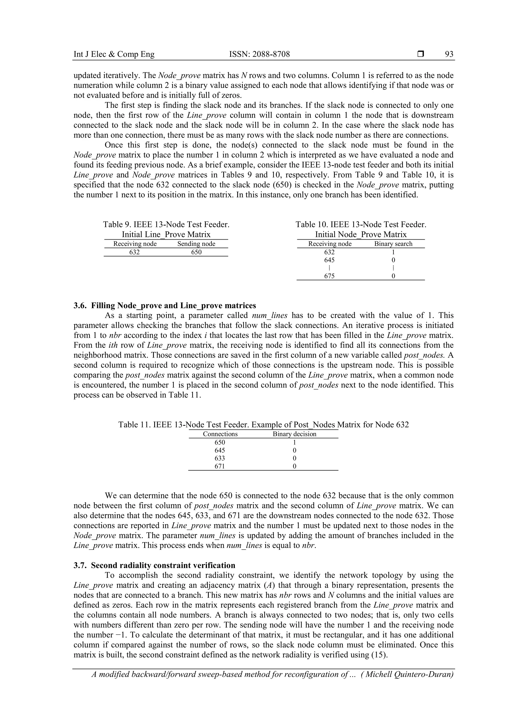
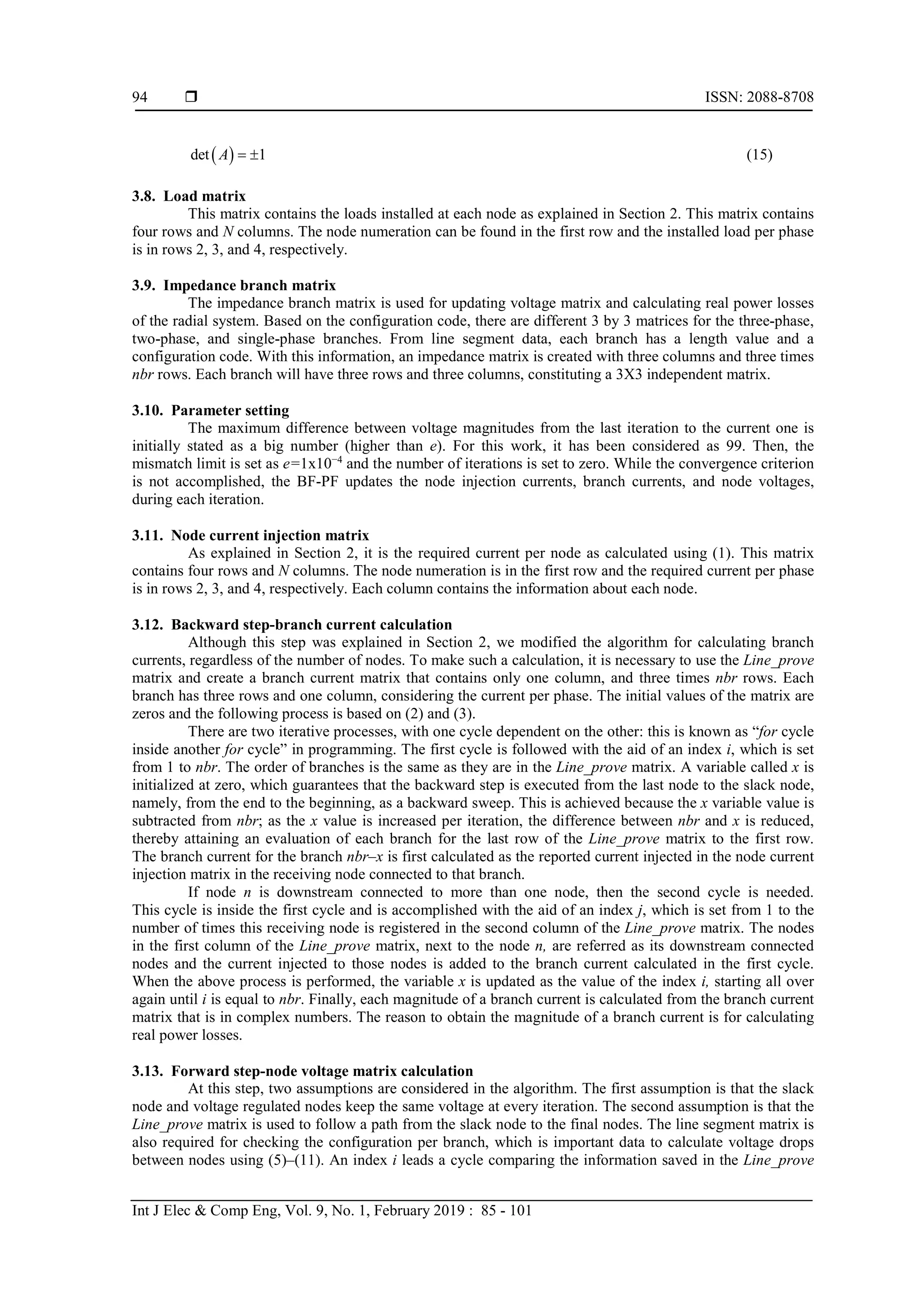
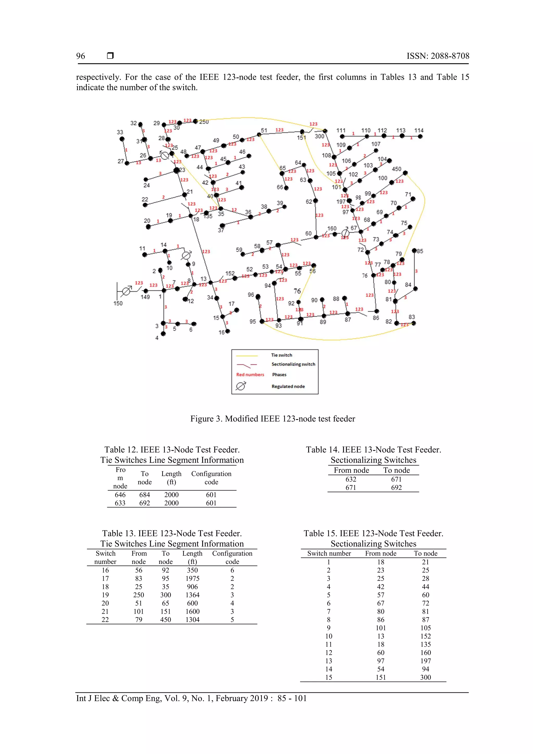
  Int J Elec& Comp Eng ISSN: 2088-8708  A modified backward/forward sweep-based method for reconfiguration of ... ( Michell Quintero-Duran) 95 matrix against the line segment matrix to obtain the number of phases of each branch. Depending on the connected phases, the algorithm must use one of (5)–(11). This algorithm saves two voltage matrices: the last iteration voltage matrix and the current iteration voltage matrix. 3.14. Convergence requirement The convergence requirement is defined because a minimum error must be reached to determine if the calculations are correct and gives a stop criterion to the algorithm to finish all the process. From last step, two voltage matrices were obtained from last iteration and current iteration. The absolute value of the magnitude difference between each pair of rows of those two matrices is calculated and saved in a matrix called the “mismatch matrix.” The maximum encountered value in this matrix is compared with the mismatch limit e as presented in (12) and set as 1x10−4 . If convergence is not reached, then the voltage matrix for the last iteration is updated with the values of the voltage matrix at the current iteration and the resulting matrix is finally ready to be used in the next iteration; otherwise, the algorithm finds the final convergence and the algorithm stops. 4. TEST FEEDERS FOR RECONFIGURATION IMPLEMENTATION There are four distribution test cases developed by Kersting for the IEEE in [29] and [30] (IEEE 13, 34, 37, and 123-node distribution test feeders). In this work, we have selected the smallest test feeder (13-node test feeder) and largest test feeder (123-node test feeder) and modified them by adding switches connected to some nodes. Figure 2 and Figure 3 show the modifications applied to the two test cases based on [32] and [33]. Figure 2. Modified IEEE 13-node test feeder From Figure 2 and Figure 3, it can be observed that there are tie and sectionalizing switches. A tie switch is a normally opened switch, and all must be three-phase to allow for a reconfiguration process; meanwhile, a sectionalizing switch is a normally closed switch. In both figures, the numbers in red refer to the phases per branch, where 123 means that phases a, b, and c are connected through the branch, where 12 means that phases a and b are connected through the branch, and so on. The regulated nodes have a regulator installed that is capable of maintaining constant voltage in that node. Information about the tie switches, added to the distribution networks for the 13-node test feeder and the 123-node test feeder, are presented in Table 12 and Table 13, respectively. Lengths and configuration of switches were calculated using the distance to the neighboring nodes. Sectionalizing switch lengths and configurations are already in the line segment matrix of each case study, although the nodes where they are connected are in Table 14 and Table 15 for the IEEE 13-node test feeder and IEEE 123-node test feeder,
• 12.
   ISSN: 2088-8708 IntJ Elec & Comp Eng, Vol. 9, No. 1, February 2019 : 85 - 101 96 respectively. For the case of the IEEE 123-node test feeder, the first columns in Tables 13 and Table 15 indicate the number of the switch. Figure 3. Modified IEEE 123-node test feeder Table 12. IEEE 13-Node Test Feeder. Tie Switches Line Segment Information Fro m node To node Length (ft) Configuration code 646 684 2000 601 633 692 2000 601 Table 14. IEEE 13-Node Test Feeder. Sectionalizing Switches From node To node 632 671 671 692 Table 13. IEEE 123-Node Test Feeder. Tie Switches Line Segment Information Switch number From node To node Length (ft) Configuration code 16 56 92 350 6 17 83 95 1975 2 18 25 35 906 2 19 250 300 1364 3 20 51 65 600 4 21 101 151 1600 3 22 79 450 1304 5 Table 15. IEEE 123-Node Test Feeder. Sectionalizing Switches Switch number From node To node 1 18 21 2 23 25 3 25 28 4 42 44 5 57 60 6 67 72 7 80 81 8 86 87 9 101 105 10 13 152 11 18 135 12 60 160 13 97 197 14 54 94 15 151 300
• 13.
  Int J Elec& Comp Eng ISSN: 2088-8708  A modified backward/forward sweep-based method for reconfiguration of ... ( Michell Quintero-Duran) 97 5. RESULTS AND DISCUSSION In this section, we present the results for different combinations of switches in both the IEEE 13-node and IEEE 123-node test feeders to demonstrate the effectiveness of the proposed modifications to the BF-PF. For the smallest case, all possible combinations of switches are recorded. However, for the largest case, the number of possible combinations is 4,194,304 and feasible combinations number 497,420; thus, we listed only the best 20 combinations. 5.1. Results for the modified IEEE 13-node test feeder The modified IEEE 13-node test feeder has four switches, indicating that the possible number of combinations is 16 as the expression for obtaining the number of combinations in a binary decision variable is calculated from (16), where n indicates the number of switches installed in the system [34]. 2n comb  (16) Table 16 shows the results for all possible combinations. The opened switches for every case are in column 1 while the real power losses are in column 2. If a combination is not feasible, then the algorithm displays a message that allows us to know exactly what constraint is not fulfilled. Table 16. IEEE 13-node test feeder. Evaluation of the Modified BF-PF Opened switches Losses (kW) All Constraint: Minimum number of branches 646-684, 633-692, 671-692 Constraint: Minimum number of branches 646-684, 633-692, 632-671 Constraint: Minimum number of branches 646-684, 633-692 102,98 646-684, 671-692, 632-671 Constraint: Minimum number of branches 646-684, 671-692 73,61 646-684, 632-671 125,78 646-684 Constraint: Minimum number of branches 633-692, 671-692, 632-671 Constraint: Minimum number of branches 633-692, 671-692 Constraint: Not feeding all nodes 633-692, 632-671 109,83 633-692 Constraint: Minimum number of branches 671-692, 632-671 68,43 671-692 Constraint: Minimum number of branches 632-671 Constraint: Minimum number of branches None Constraint: Minimum number of branches Five combinations could fulfill radiality constraints and reach the convergence requirement. The best combination for minimal real power losses is when the switches between nodes 671–692 and nodes 632–671 are opened, obtaining a total real power loss of 68.43 kW. This test feeder is easy to evaluate because it does not require large computational resources to calculate the power flow for the small number of combinations. The unfeasible combinations are separated into two groups. The first group corresponds to the configurations that obtain the number of branches different than calculated in (14), preventing to perform the power flow. The second group corresponds to the configurations that do not feed all nodes, which is the case when switches between nodes 633–692 and between 671–692 are opened, and node 675 is isolated. For this case study, the modified BF-PF can accomplish good results, allowing its use for small-scale radial unbalanced distribution networks. Aditionally, the five feasible combinations obtained with the IEEE 13-node test feeder were compared to validate the effectiveness of the Modified BF-PF (MBF-PF) against a Standard BF-PF (SBF-PF) [27]. Such comparison is presented in Table 17. Table 17. Comparison between MBF-PF and SBF-PF (IEEE 13-Node Test Feeder) Opened switches MBF-PF response SBF-PF response 646-684, 633-692 Converge Does not converge 646-684, 671-692 Converge Does not converge 646-684, 632-671 Converge Does not converge 633-692, 632-671 Converge Does not converge 671-692, 632-671 Converge Does not converge
• 14.
   ISSN: 2088-8708 IntJ Elec & Comp Eng, Vol. 9, No. 1, February 2019 : 85 - 101 98 From Table 17, it is clear that the SBF-PF does not find a solution for network reconfiguration, because it needs the special numeration considered in the MBF-PF. This result probes that the MBF-PF can find solutions for reconfiguration regardless the numeration of nodes. 5.2. Results for the modified IEEE 123-node test feeder The modified IEEE 123-node test feeder is a large-scale radial unbalanced distribution network. From Table 13 and Table 15 it is observed that there are 22 switches. Hence, 13 switches must be closed and 9 switches must be opened to fulfill radiality constraints. There are 4,194,304 combinations to evaluate, but to obtain only the feasible combinations, which number is 497,420. (17) can be used [34], where perm is the number of permutations, n the total number of switches, and r the number of whichever required opened or closed switches (as this equation is symmetric). The symbol (!) refers to the factorial value.   ! ! ! n perm r n r   (17) Despite the feasible combinations is 11.86% of the total possible combinations it is still a very large effort to evaluate all combinations in reasonable time for a real operation system case. Reconfiguration is a challenge to large-scale radial unbalanced distribution networks. We evaluated all feasible combinations using the proposed algorithm in an AMD A10-5745M APU with Radeon(tm) HD Graphics 2.10 GHz, 8 GB RAM computer in 36,022.39 seconds (approximately 10 hours). The best 20 combinations are reported in Table 18, which contains the 22 switches listed as they are in Table 13 and Table 15. When a switch is closed, the number 1 appears below the number of that switch, otherwise 0. The real power losses for each configuration are shown in the last column. Table 18. IEEE 123-Node Test Feeder. Evaluation of the Modified BF-PF. Best 20 Combinations State of switches: 0 for opened, 1 for closed Losses (kW) 1 2 3 4 5 6 7 8 9 10 11 12 13 14 15 16 17 18 19 20 21 22 1 1 1 1 1 0 0 1 1 1 1 1 1 1 0 0 1 0 0 0 0 0 204,16 1 1 1 1 1 0 0 1 1 1 1 1 0 1 0 0 1 0 1 0 0 0 204,89 1 1 1 1 1 0 0 1 0 1 1 1 1 1 0 0 1 0 1 0 0 0 205,18 1 0 1 1 1 0 0 1 1 1 1 1 1 1 0 0 1 1 0 0 0 0 205,77 1 1 1 1 1 0 0 1 0 1 1 1 0 1 0 0 1 0 1 0 1 0 206,07 0 1 1 1 1 0 0 1 1 1 1 1 1 1 0 0 1 1 0 0 0 0 206,62 1 1 1 1 1 0 1 1 1 1 1 1 1 1 0 0 0 0 0 0 0 0 207,09 1 1 1 1 1 0 0 1 1 1 1 1 1 0 0 1 1 0 0 0 0 0 207,21 1 1 1 1 1 0 1 1 1 1 1 1 0 1 0 0 0 0 1 0 0 0 207,80 1 1 1 1 1 0 0 1 1 1 1 1 0 0 0 1 1 0 1 0 0 0 207,92 1 1 1 1 1 0 1 1 0 1 1 1 1 1 0 0 0 0 1 0 0 0 208,09 1 1 1 1 1 0 0 1 0 1 1 1 1 0 0 1 1 0 1 0 0 0 208,21 1 1 1 1 1 0 0 1 0 1 1 1 1 1 1 0 1 0 0 0 0 0 208,48 1 0 1 1 1 0 1 1 1 1 1 1 1 1 0 0 0 1 0 0 0 0 208,70 1 0 1 1 1 0 0 1 1 1 1 1 1 0 0 1 1 1 0 0 0 0 208,82 From Table 18, it is observed that the best configuration for minimizing the real power losses is to keep the switches from nodes 67 and 72, 80 and 81, 151 and 300, 56 and 92, 25 and 35, 250 and 300, 51 and 65, 101 and 151, 79 and 450 opened. When an unfeasible combination is evaluated, the algorithm prompts the same message errors as those reported in Table 16. The worst scenario presented in Table 18 is 2.28% higher than the best combination obtained with the complete evaluation performed for all feasible combinations. This result means that the algorithm is capable to find good solutions with least amount of combinations leaded by a random process bounded by natural processes. Aditionally, the comparison between MBF-PF and SBF-PF [27] shows that the SBF-PF could not find the solutions to the same combinations, because it requires to renumber all the nodes for each evaluation proposed for the network reconfiguration. 6. CONCLUSION The standard BF-PF is a known algorithm for evaluating power flow in distribution systems. Some tools developed by researchers follow a strict order in node numeration. If that numeration order is changed,
• 15.
  Int J Elec& Comp Eng ISSN: 2088-8708  A modified backward/forward sweep-based method for reconfiguration of ... ( Michell Quintero-Duran) 99 then the standard BF-PF is not capable to reach the convergence requirement or even evaluate the power flow. To avoid this complication, the authors have proposed a modified BF-PF algorithm that carries a binary search from the substation node to the last node in the system. This is accomplished with the aid of several matrices that guarantee that the substation or slack node will always be the root of the tree search process, obtaining a path whereby the current is flowing. This purpose was proven on two known benchmarks from the IEEE: the IEEE 13-node test feeder and the IEEE 123-node test feeder. With these evaluations, the authors could demonstrate that with these developed modifications, this algorithm becomes a powerful tool to tackle both small- and large-scale radial unbalanced distribution networks, regardless the numeration of the nodes. Modifications on case studies were presented to evaluate different topologies in each test feeder, considering both feasible and unfeasible combinations. The algorithm was capable to evaluate every single combination and, when an unfeasible combination was evaluated, a message prompted showing what constraint was not fulfilled by the configuration. The authors also introduced a permutation equation for obtaining only feasible combinations. This allows making power flows in a reconfiguration process while avoiding unfeasible combinations. The results for each case study were presented and analyzed to comment the effectiveness of the proposed modifications. ACKNOWLEDGEMENTS The authors thank to the Colombian Departamento Administrativo de Ciencia, Tecnologia e Innovacion (Administrative Department of Science, Technology and Innovation) – Colciencias for the necessary resources to pursue the PhD program on Engineering at the Universidad Nacional de Colombia and to this Research through the call number 727 from 2015. To the Universidad Nacional de Colombia for offering working spaces and professional evaluations to carry this investigation. And to the Universidad de la Costa for sponsoring the main author to pursue his PhD program and research. REFERENCES [1] C. Harrap, X. Bai, Y. Mavrocostanti, and D. Strickland, “Distribution Network Reconfiguration Validation with Uncertain Loads – Network Configuration Determination And Application,” IET Gener. Transm. Distrib., vol. 10, no. 12, pp. 2852–2860, Sep. 2016. [2] E. Herazo, M. Quintero, J. Candelo, J. Soto, and J. Guerrero, “Optimal Power Distribution Network Reconfiguration Using Cuckoo Search,” in 2015 4th International Conference on Electric Power and Energy Conversion Systems (EPECS), 2015, pp. 1–6. [3] T. Niknam, A. Kavousi Fard, and A. Baziar, “Multi-Objective Stochastic Distribution Feeder Reconfiguration Problem Considering Hydrogen and Thermal Energy Production by Fuel Cell Power Plants,” Energy, vol. 42, no. 1, pp. 563–573, Jun. 2012. [4] M. M. Aman, G. B. Jasmon, A. H. Abu Bakar, H. Mokhlis, and K. Naidu, “Graph Theory-Based Radial Load Flow Analysis to Solve the Dynamic Network Reconfiguration Problem,” Int. Trans. Electr. Energy Syst., vol. 26, no. 4, pp. 783–808, Apr. 2016. [5] D. R. R. Penido, L. R. de Araujo, S. Carneiro Júnior, and J. L. R. Pereira, “A New Tool for Multiphase Electrical Systems Analysis Based on Current Injection Method,” Int. J. Electr. Power Energy Syst., vol. 44, no. 1, pp. 410– 420, Jan. 2013. [6] M. Quintero-Duran, J. E. Candelo, and V. Sousa, “Recent Trends of the Most Used Metaheuristic Techniques for Distribution Network Reconfiguration,” J. Eng. Sci. Technol. Rev., vol. 10, no. 5, pp. 159–173, 2017. [7] D. Rajicic, R. Ackovski, and R. Taleski, “Voltage Correction Power Flow,” IEEE Trans. Power Deliv., vol. 9, no. 2, pp. 1056–1062, Apr. 1994. [8] U. Ghatak and V. Mukherjee, “An Improved Load Flow Technique Based On Load Current Injection for Modern Distribution System,” Int. J. Electr. Power Energy Syst., vol. 84, pp. 168–181, Jan. 2017. [9] U. Ghatak and V. Mukherjee, “A Fast And Efficient Load Flow Technique For Unbalanced Distribution System,” Int. J. Electr. Power Energy Syst., vol. 84, pp. 99–110, Jan. 2017. [10] Jin-Cheng Wang, Hsiao-Dong Chiang, and G. R. Darling, “An Efficient Algorithm for Real-Time Network Reconfiguration in Large Scale Unbalanced Distribution Systems,” IEEE Trans. Power Syst., vol. 11, no. 1, pp. 511–517, 1996. [11] J.-C. Wang, H.-D. Chiang, and G. R. Darling, “Efficient Algorithm for Real-Time Network Reconfiguration in Large Scale Unbalanced Distribution Systems,” in IEEE Power Industry Computer Applications Conference, 1995, pp. 510–516. [12] G. Diaz, J. Gomez-Aleixandre, and J. Coto, “Direct Backward/Forward Sweep Algorithm for Solving Load Power Flows in AC Droop-Regulated Microgrids,” IEEE Trans. Smart Grid, vol. 7, no. 5, pp. 2208–2217, Sep. 2016. [13] H. Cun, T. Yongjie, and H. Fei, “A Fuzzy Power Flow Calculation Based On Forward-Backward Sweep Method,” in 2016 Chinese Control and Decision Conference (CCDC), 2016, pp. 3118–3123. [14] R. J. R. Kumar and A. Jain, “Power Loss and Voltage Regulation Calculation in A Radial System with Distributed Generations and Voltage Regulators,” in 2015 International Conference on Energy, Power and Environment:
• 16.
   ISSN: 2088-8708 IntJ Elec & Comp Eng, Vol. 9, No. 1, February 2019 : 85 - 101 100 Towards Sustainable Growth (ICEPE), 2015, pp. 1–5. [15] Nimal Madhu M, N. Sasidharan, and J. G. Singh, “A Droop Control Incorporated Dc Equivalent Power Flow Method For Distribution and Low Voltage Systems,” Electr. Power Syst. Res., vol. 134, pp. 56–65, May 2016. [16] P. Wirasanti and E. Ortjohann, “Active Distribution Grid Power Flow Analysis using Asymmetrical Hybrid Technique,” Int. J. Electr. Comput. Eng., vol. 7, no. 4, p. 1738, Aug. 2017. [17] D. Issicaba and J. Coelho, “Convergence Evaluation of a Load Flow Method based on Cespedes’ Approach to Distribution System Analysis,” Int. J. Electr. Comput. Eng., vol. 6, no. 6, p. 3276, Dec. 2016. [18] D. Issicaba and J. Coelho, “Rotational Load Flow Method for Radial Distribution Systems,” Int. J. Electr. Comput. Eng., vol. 6, no. 3, p. 1344, Jun. 2016. [19] D. Issicaba and J. Coelho, “Evaluation of the Forward-Backward Sweep Load Flow Method using the Contraction Mapping Principle,” Int. J. Electr. Comput. Eng., vol. 6, no. 6, p. 3229, Dec. 2016. [20] K. Sunderland, M. Coppo, M. Conlon, and R. Turri, “A Correction Current Injection Method for Power Flow Analysis Of Unbalanced Multiple-Grounded 4-Wire Distribution Networks,” Electr. Power Syst. Res., vol. 132, pp. 30–38, Mar. 2016. [21] Maya K N and E. A. Jasmin, “A Generalised Three Phase Power Flow Algorithm Incorporating the Uncertainty of Photo Voltaic(PV) Source for Unbalanced Distribution Network,” in 2015 International Conference on Technological Advancements in Power and Energy (TAP Energy), 2015, pp. 29–34. [22] P. Samal and S. Ganguly, “A Modified Forward Backward Sweep Load Flow Algorithm for Unbalanced Radial Distribution Systems,” in 2015 IEEE Power & Energy Society General Meeting, 2015, vol. 2015–Septe, pp. 1–5. [23] C. P. Nguyen and A. J. Flueck, “A Novel Agent-Based Distributed Power Flow Solver for Smart Grids,” IEEE Trans. Smart Grid, vol. 6, no. 3, pp. 1261–1270, May 2015. [24] Y. Ju, W. Wu, and B. Zhang, “Convergence Problem in Forward/Backward Sweep Power Flow Method Caused by Non-Positive-Sequence Impedance of Distributed Generators and Its Solution,” Int. J. Electr. Power Energy Syst., vol. 65, pp. 463–466, Feb. 2015. [25] B. B. Navarro, D. A. H. O. Asakil, and M. M. Navarro, “Medium Voltage to Low Voltage Power Flow Solution Using Modified Backward/Forward Sweep Algorithm,” in IECON 2015 - 41st Annual Conference of the IEEE Industrial Electronics Society, 2015, pp. 001115–001120. [26] F. Xue, W. Xie, P. Xie, Z. Pan, J. Ren, Y. Nie, X. Wang, and M. Chen, “Unbalanced Three-Phase Distribution System Power Flow With Distributed Generation Using Affine Arithmetic,” in 2015 5th International Conference on Electric Utility Deregulation and Restructuring and Power Technologies (DRPT), 2015, pp. 822–829. [27] S. Mishra, “A Simple Algorithm For Unbalanced Radial Distribution System Load Flow,” in TENCON 2008 - 2008 IEEE Region 10 Conference, 2008, pp. 1–6. [28] J. B. V Subrahmanyam and C. Radhakrishna, “A Simple Method for Feeder Reconfiguration of Balanced and Unbalanced Distribution Systems for Loss Minimization,” Electr. Power Components Syst., vol. 38, no. 1, pp. 72– 84, Dec. 2009. [29] W. Kersting, “Radial Distribution Test Feeders,” in Proceedings of the IEEE Power Engineering Society Transmission and Distribution Conference, 2001, vol. 2, no. WINTER MEETING, pp. 908–912. [30] W. H. Kersting, “Radial Distribution Test Feeders,” IEEE Trans. Power Syst., vol. 6, no. 3, pp. 975–985, 1991. [31] W. Kersting, Distribution System Modeling and Analysis. New Mexico, 2002. [32] W. H. Kersting, “The Simulation of Loop Flow in Radial Distribution Analysis Programs,” in 2014 IEEE Rural Electric Power Conference (REPC), 2014, pp. B3-1-B3-6. [33] S. Wang and H.-D. Chiang, “Multi-Objective Service Restoration of Distribution Systems Using User-Centered Methodology,” Int. J. Electr. Power Energy Syst., vol. 80, pp. 140–149, Sep. 2016. [34] D. C. Montgomery, Design and Analysis of Experiments, vol. 48, no. 1. 2006. BIOGRAPHIES OF AUTHORS Michell Josep Quintero Duran received his Bs. degree in Electrical Engineering in 2013 from Universidad de la Costa, Barranquilla – Colombia, and his MSc degree in Electrical Engineering in 2017 from Universidad del Norte, Baranquilla – Colombia. He is currently pursuing his PhD program on Engineering with emphasis in Energy Systems. His employment experiences include the Universidad del Norte and Universidad de la Costa. He is now a Full-Time Professor of the Universidad de la Costa. His research interests include operation and control of power systems, renewable energies, and artificial intelligence. ORCID: 0000-0003-1406-9888
• 17.
  Int J Elec& Comp Eng ISSN: 2088-8708  A modified backward/forward sweep-based method for reconfiguration of ... ( Michell Quintero-Duran) 101 John Edwin Candelo received his Bs. degree in Electrical Engineering in 2002 and his PhD in Engineering with emphasis in Electrical Engineering in 2009 from Universidad del Valle, Cali - Colombia. His employment experiences include the Empresa de Energía del Pacífico EPSA, Universidad del Norte, and Universidad Nacional de Colombia. He is now an Assistant Professor of the Universidad Nacional de Colombia, Medellín, Colombia. His research interests include: planning, operation and control of power systems, artificial intelligence, and smart grids. ORCID: 0000-0002-9784-9494 José Daniel Soto Ortiz received his B.S. degree and Ph.D in electrical engineering from Georgian Technical University, USSR. He is currently working at Universidad del Norte in Barranquilla, Colombia and his research interests include high voltage engineering and renewable energy. ORCID: 0000-0002-1143-7844