If You’ve Never Used Excel’s FILTER Function, You’re Seriously Missing Out

If you're still manually sifting through massive spreadsheets or relying on clunky, old-school sorting tools, you're doing it the hard way. Excel has the powerful FILTER function, a built-in solution that you've likely overlooked.

What Is the FILTER Function in Excel

The FILTER function is a dynamic array formula that automatically extracts rows from your data based on specific criteria. Instead of using methods to sort and filter data by color, this function creates a live, updating list that changes whenever your source data changes.

Here's the basic syntax:

=FILTER(array, include, [if_empty])

The array is your data range, include defines your criteria, and if_empty shows a custom message when no results match.

The dynamic behavior is its key advantage. When you change a value in your source data, the filtered results update instantly, so you don't need to refresh afterward. Hence, it beats static filtering methods that require manual updates every time your data changes.

The FILTER function works with text, numbers, and dates. You can filter sales data by region, find employees hired after a specific date, or extract products above a certain price point. You can even combine it with other functions to perform basic math in Excel on your filtered results.

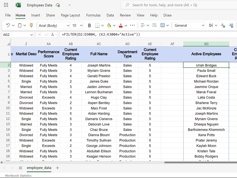
Let's say you're an HR manager who needs to identify all active employees quickly. Instead of scrolling through 3,000+ employee records, you can use:

=FILTER(D2:D3004, (K2:K3004="Active"))

This formula utilizes the FILTER function to display only active employees and eliminates the need to do any manual sorting.

Advanced FILTER Tricks for Power Users

Once you master basic filtering, you can combine multiple criteria, which opens up more possibilities for data analysis. Unlike simple data filtering in tables, advanced FILTER techniques let you build complex logic that mirrors business decisions.

Filtering With AND Logic

AND logic requires every condition to be met simultaneously. Here, we use the asterisk (*) operator to multiply logical tests together. Each condition acts as a gate that data must pass through.

As an example of employee data, the following formula will return only those employees who are active, work in sales, and are full-time.

=FILTER(A2:AC3004, (K2:K3004="Active") * (Q2:Q3004="Sales") * (L2:L3004="Full-Time"))

All three conditions must be true for an employee to appear in your results. If one condition is missed, the employee gets filtered out entirely. This approach works perfectly when you need to narrow down candidates for specific roles or compliance requirements.

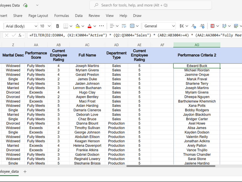
You can stack as many AND conditions as needed, such as adding performance criteria to find active sales employees with high ratings and who fully meet the requirements.

=FILTER(D2:D3004, (K2:K3004="Active") * (Q2:Q3004="Sales") * (AB2:AB3004>=4) * (AA2:AA3004="Fully Meets"))

Filtering With OR Logic

OR logic yields results when any one of the conditions is met. In this case, we use the plus (+) operator between logical tests.

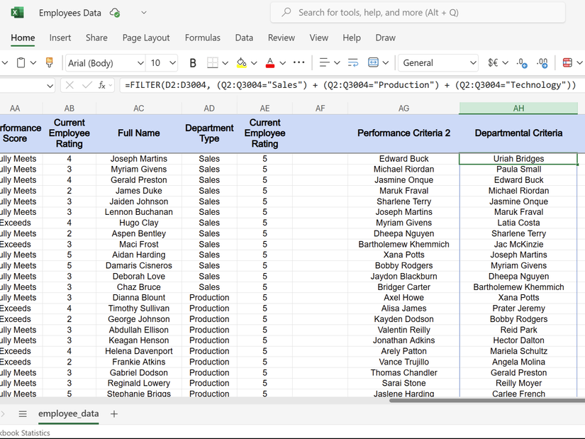
=FILTER(D2:D3004, (Q2:Q3004="Sales") + (Q2:Q3004="Production") + (Q2:Q3004="Technology"))

The above formula filters employees from sales, production, or technology departments. Unlike AND filtering, meeting just one condition is sufficient to qualify a record for inclusion. So, OR logic expands your results rather than narrowing them.

This type of filtering is useful when you're casting a wider net. For instance, if you need employees from multiple departments for a cross-functional project, you can use OR logic to capture everyone relevant without requiring separate formulas for each department.

Combining AND and OR Logic

You can mix AND and OR logic for complex queries. If you want high-performing employees from key departments, then you can try the following combination.

=FILTER(A2:AC3004, ((Q2:Q3004="Sales") + (Q2:Q3004="Production")) * (AB2:AB3004>=4))

This formula finds employees in sales or production who have performance ratings of four or higher. The parentheses control the order of operations, just like mathematical equations.

You can even apply this in more complex scenarios, like filtering terminated employees for specific reasons. Such a combined formula can capture employees who left voluntarily or were terminated for cause, but only those with termination descriptions filled in.

Understanding how these logical operators work together can be handy for advanced data analysis capabilities that reduce spreadsheet chaos into actionable insights.

Common FILTER Function Pitfalls to Avoid

Even experienced Excel users stumble when first using FILTER. These common mistakes can derail your formulas, but they're easy to fix once you know what to watch for.

The #SPILL! Error

This error appears when your filtered results can't be displayed because other data blocks their path. FILTER creates dynamic arrays that need empty space to expand. To fix this, clear any data below and to the right of your formula cell.

If you're filtering 50 employees but only have 10 empty rows available, Excel throws #SPILL! error instead of showing partial results. Always ensure adequate space for your maximum possible output.

Mismatched Data Types

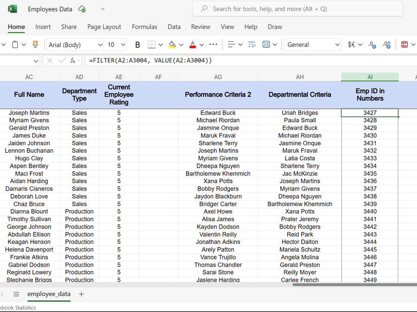
Text that resembles numbers can sometimes break FILTER logic. Employee IDs stored as text won't match numeric criteria. I use the following formula to convert text-based employee IDs to numbers before filtering.

=FILTER(A2:A3004, VALUE(A2:A3004))

Similarly, dates formatted as text require conversion—wrap date columns with DATEVALUE() to ensure proper comparison.

=FILTER(A2:AC3004, DATEVALUE(E2:E3004)>=DATE(2020,1,1))

Case Sensitivity Issues

FILTER treats "Sales" and "sales" as different values. Convert text case in Excel by using a function like UPPER() or LOWER() to standardize text before comparison. This catches variations in data entry that would otherwise slip through your filters.

=FILTER(A2:AC3004, UPPER(Q2:Q3004)="SALES")

Range Size Mismatches

Your criteria range must match your data range exactly. If your data spans A2:AC3004 but your criteria references K2:K3000, you'll miss four rows of data—potentially important records.

Always double-check that your ranges align. Use Ctrl + Shift + End to find your actual data boundaries rather than guessing where your data ends.

Handling Empty Results

When no data matches your criteria, FILTER returns #CALC! by default. Therefore, you must use the third parameter to display custom messages. This creates cleaner reports and prevents confusion when sharing filtered data with colleagues who might not understand Excel error messages.

=FILTER(A2:AC3004, K2:K3004="Future Start", "No future employees found")

Performance With Large Datasets

FILTER recalculates every time your source data changes. With thousands of rows and multiple criteria, this can cause Excel to slow to a crawl. Consider using manual calculation mode by using the shortcut Ctrl + Alt + F9 when working with large datasets.

For recurring reports, copy and paste filtered results as values instead of keeping live formulas. Doing so reduces file size and improves performance while preserving your analyzed data.

---

Excel offers plenty of ways to organize data, but FILTER delivers instant, dynamic results without the hassle. Once you experience real-time filtering that updates automatically, you'll not look back.