Feature Engineering: Scaling, Normalization and Standardization
Last Updated : 17 Sep, 2025
Feature engineering is the process of creating, transforming or selecting the most relevant variables (features) from raw data to improve model performance. Effective features help the model capture important patterns and relationships in the data. It directly contributes to model building in the following ways:
- Well-designed features allow models to learn complex patterns more effectively.
- Reduces noise and irrelevant information, improving prediction accuracy.
- Helps prevent overfitting by emphasizing meaningful data signals.
- Simplifies model interpretation by creating more informative and understandable inputs.
There are various techniques, such as scaling, normalization and standardization that can be used for feature engineering. Let's explore some of them.
1. Absolute Maximum Scaling
Absolute Maximum Scaling rescales each feature by dividing all values by the maximum absolute value of that feature. This ensures the feature values fall within the range of -1 to 1. While simple and useful in some contexts, it is highly sensitive to outliers which can skew the max absolute value and negatively impact scaling quality.
X_{\rm {scaled }}=\frac{X_{i}}{\rm{max}\left(|X|\right)}
- Scales values between -1 and 1.
- Sensitive to outliers, making it less suitable for noisy datasets.
Code Example: We will first Load the Dataset
Dataset can be downloaded from here.
Python import pandas as pd import numpy as np df = pd.read_csv('Housing.csv') df = df.select_dtypes(include=np.number) df.head() Output:
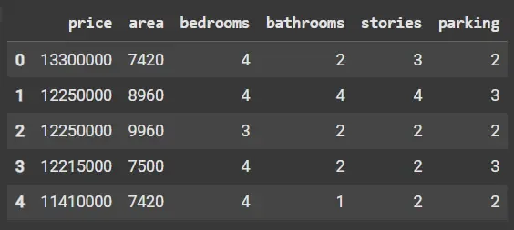 Dataset
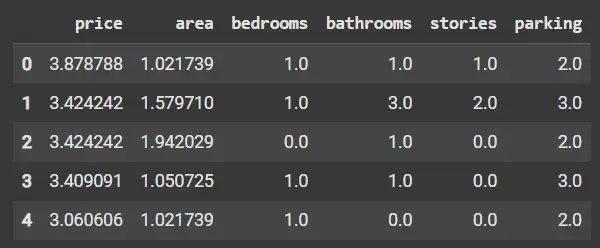
Performing Absolute Maximum Scaling
- Computes max absolute value per column with np.max(np.abs(df), axis=0).
- Divides each value by that max absolute to scale features between -1 and 1.
- Displays first few rows of scaled data with scaled_df.head().
Python max_abs = np.max(np.abs(df), axis=0) scaled_df = df / max_abs scaled_df.head()
Output:
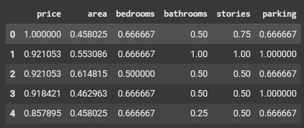 Absolute Maximum Scaling
2. Min-Max Scaling
Min-Max Scaling transforms features by subtracting the minimum value and dividing by the difference between the maximum and minimum values. This method maps feature values to a specified range, commonly 0 to 1, preserving the original distribution shape but is still affected by outliers due to reliance on extreme values.
X_{\rm {scaled }}=\frac{X_{i}-X_{\text {min}}}{X_{\rm{max}} - X_{\rm{min}}}
- Scales features to range.
- Sensitive to outliers because min and max can be skewed.
Code Example: Performing Min-Max Scaling
- Creates MinMaxScaler object to scale features to range.
- Fits scaler to data and transforms with scaler.fit_transform(df).
- Converts result to DataFrame maintaining column names.
- Shows first few scaled rows with scaled_df.head().
Python from sklearn.preprocessing import MinMaxScaler scaler = MinMaxScaler() scaled_data = scaler.fit_transform(df) scaled_df = pd.DataFrame(scaled_data, columns=df.columns) scaled_df.head()
Output:
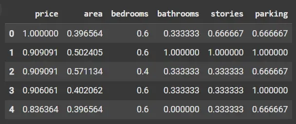 Min-Max Scaling
3. Normalization (Vector Normalization)
Normalization scales each data sample (row) such that its vector length (Euclidean norm) is 1. This focuses on the direction of data points rather than magnitude making it useful in algorithms where angle or cosine similarity is relevant, such as text classification or clustering.
X_{\text{scaled}} = \frac{X_i}{\| X \|}
Where:
- {X_i} is each individual value.
- {\| X \|} represents the Euclidean norm (or length) of the vector X.
- Normalizes each sample to unit length.
- Useful for direction-based similarity metrics.
Code Example: Performing Normalization
- Scales each row (sample) to have unit norm (length = 1) based on Euclidean distance.
- Focuses on direction rather than magnitude of data points.
- Useful for algorithms relying on similarity or angles (e.g., cosine similarity).
- scaled_df.head() shows normalized data where each row is scaled individually.
Python from sklearn.preprocessing import Normalizer scaler = Normalizer() scaled_data = scaler.fit_transform(df) scaled_df = pd.DataFrame(scaled_data, columns=df.columns) scaled_df.head()
Output:
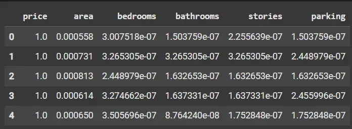 Normalization
4. Standardization
Standardization centers features by subtracting the mean and scales them by dividing by the standard deviation, transforming features to have zero mean and unit variance. This assumption of normal distribution often benefits models like linear regression, logistic regression and neural networks by improving convergence speed and stability.
X_{\rm {scaled }}=\frac{X_{i}-\mu}{\sigma}
- where \mu = mean, \sigma = standard deviation.
- Produces features with mean 0 and variance 1.
- Effective for data approximately normally distributed.
Code Example: Performing Standardization
- Centers features by subtracting mean and scales to unit variance.
- Transforms data to have zero mean and standard deviation of 1.
- Assumes roughly normal distribution; improves many ML algorithms’ performance.
- scaled_df.head() shows standardized features.
Python from sklearn.preprocessing import StandardScaler scaler = StandardScaler() scaled_data = scaler.fit_transform(df) scaled_df = pd.DataFrame(scaled_data, columns=df.columns) print(scaled_df.head())
Output:
 Standardization
5. Robust Scaling
Robust Scaling uses the median and interquartile range (IQR) instead of the mean and standard deviation making the transformation robust to outliers and skewed distributions. It is highly suitable when the dataset contains extreme values or noise.
X_{\rm {scaled }}=\frac{X_{i}-X_{\text {median }}}{IQR}
- Reduces influence of outliers by centering on median
- Scales based on IQR, which captures middle 50% spread
Code Example: Performing Robust Scaling
- Uses median and interquartile range (IQR) for scaling instead of mean/std.
- Robust to outliers and skewed data distributions.
- Centers data around median and scales based on spread of central 50% values.
- scaled_df.head() shows robustly scaled data minimizing outlier effects.
Python from sklearn.preprocessing import RobustScaler scaler = RobustScaler() scaled_data = scaler.fit_transform(df) scaled_df = pd.DataFrame(scaled_data, columns=df.columns) print(scaled_df.head())
Output:
 Robust Scaling
Comparison of Various Feature Scaling Techniques
Let's see the key differences across the five main feature scaling techniques commonly used in machine learning preprocessing.
Type | Method Description | Sensitivity to Outliers | Typical Use Cases |
|---|
Absolute Maximum Scaling | Divides values by max absolute value in each feature | High | Sparse data, simple scaling |
|---|
Min-Max Scaling (Normalization) | Scales features to by min-max normalization | High | Neural networks, bounded input features |
|---|
Normalization (Vector Norm) | Scales each sample vector to unit length (norm = 1) | Not applicable (per row) | Direction-based similarity, text classification |
|---|
Standardization (Z-Score) | Centers features to mean 0 and scales to unit variance | Moderate | Most ML algorithms, assumes approx. normal data |
|---|
Robust Scaling | Centers on median and scales using IQR | Low | Data with outliers, skewed distributions |
|---|
Advantages
- Improves Model Performance: Enhances accuracy and predictive power by presenting features in comparable scales.
- Speeds Up Convergence: Helps gradient-based algorithms train faster and more reliably.
- Prevents Feature Bias: Avoids dominance of large-scale features, ensuring fair contribution from all features.
- Increases Numerical Stability: Reduces risks of overflow/underflow in computations.
- Facilitates Algorithm Compatibility: Makes data suitable for distance- and gradient-based models like SVM, KNN and neural networks.
Explore
Machine Learning Basics
Python for Machine Learning
Feature Engineering
Supervised Learning
Unsupervised Learning
Model Evaluation and Tuning
Advanced Techniques
Machine Learning Practice
My Profile