SMS Spam Detection using TensorFlow in Python
Last Updated : 28 Jul, 2025
In today's society, practically everyone has a mobile phone, and they all get communications (SMS/ email) on their phone regularly. But the essential point is that majority of the messages received will be spam, with only a few being ham or necessary communications. Scammers create fraudulent text messages to deceive you into giving them your personal information, such as your password, account number, or Social Security number. If they have such information, they may be able to gain access to your email, bank, or other accounts.
In this article, we are going to develop various deep learning models using Tensorflow for SMS spam detection and also analyze the performance metrics of different models.
We will be using SMS Spam Detection Dataset, which contains SMS text and corresponding label (Ham or spam)
Implementation
We will import all the required libraries
Python import numpy as np import pandas as pd import matplotlib.pyplot as plt import seaborn as sns import tensorflow as tf from tensorflow import keras from tensorflow.keras import layers
Load the Dataset using pandas function .read_csv()
Python # Reading the data df = pd.read_csv("/content/spam.csv",encoding='latin-1') df.head() Lets, Understand the data

As we can see that the dataset contains three unnamed columns with null values. So we drop those columns and rename the columns v1 and v2 to label and Text, respectively. Since the target variable is in string form, we will encode it numerically using pandas function .map().
Python df = df.drop(['Unnamed: 2','Unnamed: 3','Unnamed: 4'],axis=1) df = df.rename(columns={'v1':'label','v2':'Text'}) df['label_enc'] = df['label'].map({'ham':0,'spam':1}) df.head() Output after the above data preprocessing.

Let's visualize the distribution of Ham and Spam data.
Python sns.countplot(x=df['label']) plt.show()
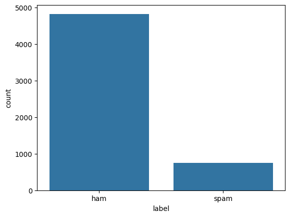 countplot
The ham data is comparatively higher than spam data, it's natural. Since we are going to use embeddings in our deep learning model, we need not balance the data. Now, let's find the average number of words in all the sentences in SMS data.
Python # Find average number of tokens in all sentences avg_words_len=round(sum([len(i.split()) for i in df['Text']])/len(df['Text'])) print(avg_words_len)
Output
16
Now, let's find the total number of unique words in the corpus
Python # Finding Total no of unique words in corpus s = set() for sent in df['Text']: for word in sent.split(): s.add(word) total_words_length=len(s) print(total_words_length)
Output
15686
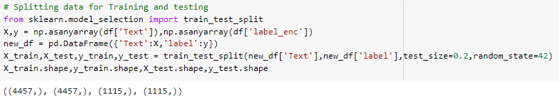
Now, splitting the data into training and testing parts using train_test_split() function.
Python # Splitting data for Training and testing from sklearn.model_selection import train_test_split X, y = np.asanyarray(df['Text']), np.asanyarray(df['label_enc']) new_df = pd.DataFrame({'Text': X, 'label': y}) X_train, X_test, y_train, y_test = train_test_split( new_df['Text'], new_df['label'], test_size=0.2, random_state=42) X_train.shape, y_train.shape, X_test.shape, y_test.shape Shape of train and test data
Building the models
First, we will build a baseline model and then we'll try to beat the performance of the baseline model using deep learning models (embeddings, LSTM, etc)
Here, we will choose MultinomialNB(), which performs well for text classification when the features are discrete like word counts of the words or tf-idf vectors. The tf-idf is a measure that tells how important or relevant a word is the document.
Python from sklearn.feature_extraction.text import TfidfVectorizer from sklearn.naive_bayes import MultinomialNB from sklearn.metrics import classification_report,accuracy_score tfidf_vec = TfidfVectorizer().fit(X_train) X_train_vec,X_test_vec = tfidf_vec.transform(X_train),tfidf_vec.transform(X_test) baseline_model = MultinomialNB() baseline_model.fit(X_train_vec,y_train)
Performance of baseline model

Confusion matrix for the baseline model

Model 1: Creating custom Text vectorization and embedding layers:
Text vectorization is the process of converting text into a numerical representation. Example: Bag of words frequency, Binary Term frequency, etc.;
A word embedding is a learned representation of text in which words with related meanings have similar representations. Each word is assigned to a single vector, and the vector values are learned like that of a neural network.
Now, we'll create a custom text vectorization layer using TensorFlow.
Python from tensorflow.keras.layers import TextVectorization MAXTOKENS=total_words_length OUTPUTLEN=avg_words_len text_vec = TextVectorization( max_tokens=MAXTOKENS, standardize='lower_and_strip_punctuation', output_mode='int', output_sequence_length=OUTPUTLEN ) text_vec.adapt(X_train)
- MAXTOKENS is the maximum size of the vocabulary which was found earlier
- OUTPUTLEN is the length to which the sentences should be padded irrespective of the sentence length.
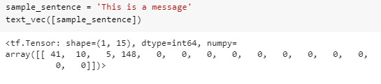
Output of a sample sentence using text vectorization is shown below:
Now let's create an embedding layer
Python embedding_layer = layers.Embedding( input_dim=MAXTOKENS, output_dim=128, embeddings_initializer='uniform', input_length=OUTPUTLEN )
- input_dim is the size of vocabulary
- output_dim is the dimension of the embedding layer i.e, the size of the vector in which the words will be embedded
- input_length is the length of input sequences
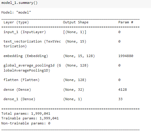
Now, let's build and compile model 1 using the Tensorflow Functional API
Python input_layer = layers.Input(shape=(1,), dtype=tf.string) vec_layer = text_vec(input_layer) embedding_layer_model = embedding_layer(vec_layer) x = layers.GlobalAveragePooling1D()(embedding_layer_model) x = layers.Flatten()(x) x = layers.Dense(32, activation='relu')(x) output_layer = layers.Dense(1, activation='sigmoid')(x) model_1 = keras.Model(input_layer, output_layer) model_1.compile(optimizer='adam', loss=keras.losses.BinaryCrossentropy( label_smoothing=0.5), metrics=['accuracy'])
Summary of the model 1
Training the model-1
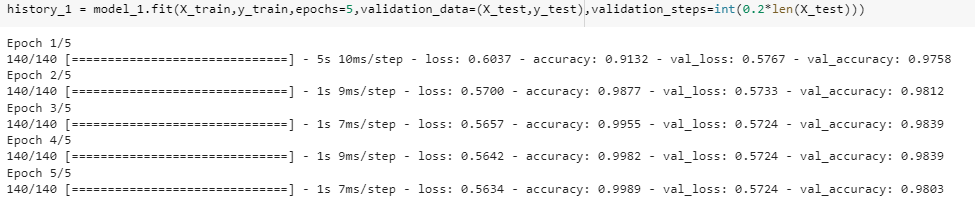
Plotting the history of model-1

Let's create helper functions for compiling, fitting, and evaluating the model performance.
Python from sklearn.metrics import precision_score, recall_score, f1_score def compile_model(model): ''' simply compile the model with adam optimzer ''' model.compile(optimizer=keras.optimizers.Adam(), loss=keras.losses.BinaryCrossentropy(), metrics=['accuracy']) def evaluate_model(model, X, y): ''' evaluate the model and returns accuracy, precision, recall and f1-score ''' y_preds = np.round(model.predict(X)) accuracy = accuracy_score(y, y_preds) precision = precision_score(y, y_preds) recall = recall_score(y, y_preds) f1 = f1_score(y, y_preds) model_results_dict = {'accuracy': accuracy, 'precision': precision, 'recall': recall, 'f1-score': f1} return model_results_dict def fit_model(model, epochs, X_train=X_train, y_train=y_train, X_test=X_test, y_test=y_test): ''' fit the model with given epochs, train and test data ''' # Check if validation data is provided if X_test is not None and y_test is not None: history = model.fit(X_train, y_train, epochs=epochs, validation_data=(X_test, y_test)) #Removed validation steps argument else: # Handle case where validation data is not provided history = model.fit(X_train, y_train, epochs=epochs) return history # This code is modified by Susobhan Akhuli Model -2 Bidirectional LSTM
A bidirectional LSTM (Long short-term memory) is made up of two LSTMs, one accepting input in one direction and the other in the other. BiLSTMs effectively improve the network's accessible information, boosting the context for the algorithm (e.g. knowing what words immediately follow and precede a word in a sentence).
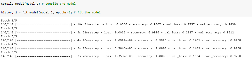
Building and compiling the model-2
Python input_layer = layers.Input(shape=(1,), dtype=tf.string) vec_layer = text_vec(input_layer) embedding_layer_model = embedding_layer(vec_layer) bi_lstm = layers.Bidirectional(layers.LSTM( 64, activation='tanh', return_sequences=True))(embedding_layer_model) lstm = layers.Bidirectional(layers.LSTM(64))(bi_lstm) flatten = layers.Flatten()(lstm) dropout = layers.Dropout(.1)(flatten) x = layers.Dense(32, activation='relu')(dropout) output_layer = layers.Dense(1, activation='sigmoid')(x) model_2 = keras.Model(input_layer, output_layer) compile_model(model_2) # compile the model history_2 = fit_model(model_2, epochs=5, X_train=X_train, y_train=y_train, X_test=X_test, y_test=y_test) # fit the model # This code is modified by Susobhan Akhuli
Training the model
Model -3 Transfer Learning with USE Encoder
Transfer Learning
Transfer learning is a machine learning approach in which a model generated for one job is utilized as the foundation for a model on a different task.
USE Layer (Universal Sentence Encoder)
The Universal Sentence Encoder converts text into high-dimensional vectors that may be used for text categorization, semantic similarity, and other natural language applications.
The USE can be downloaded from tensorflow_hub and can be used as a layer using .kerasLayer() function.
Python import tensorflow_hub as hub import tensorflow as tf from tensorflow import keras from tensorflow.keras import layers # Disable XLA compilation tf.config.optimizer.set_jit(False) # model with functional api input_layer = keras.Input(shape=[], dtype=tf.string) # universal-sentence-encoder layer # directly from tfhub use_layer = hub.KerasLayer("https://www.kaggle.com/models/google/universal-sentence-encoder/tensorFlow2/universal-sentence-encoder/2?tfhub-redirect=true", trainable=False, input_shape=[], dtype=tf.string, name='USE') # Create a Lambda layer to wrap the use_layer call # Specify the output shape of the USE layer x = layers.Lambda(lambda x: use_layer(x), output_shape=(512,))(input_layer) x = layers.Dropout(0.2)(x) x = layers.Dense(64, activation=keras.activations.relu)(x) output_layer = layers.Dense(1, activation=keras.activations.sigmoid)(x) model_3 = keras.Model(input_layer, output_layer) compile_model(model_3) history_3 = fit_model(model_3, epochs=5) # This code is modified by Susobhan Akhuli Compiling and training the model
 Training model with USE
Analyzing our Model Performance
We will use the helper function which we created earlier to evaluate model performance.
Python baseline_model_results = evaluate_model(baseline_model, X_test_vec, y_test) model_1_results = evaluate_model(model_1, X_test, y_test) model_2_results = evaluate_model(model_2, X_test, y_test) model_3_results = evaluate_model(model_3, X_test, y_test) total_results = pd.DataFrame({'MultinomialNB Model':baseline_model_results, 'Custom-Vec-Embedding Model':model_1_results, 'Bidirectional-LSTM Model':model_2_results, 'USE-Transfer learning Model':model_3_results}).transpose() total_results Output
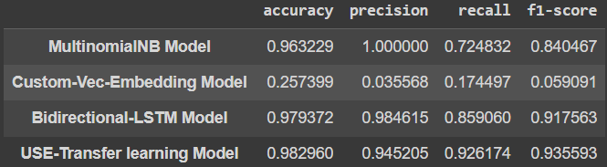 baseline model results
Plotting the results
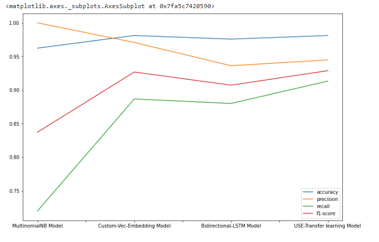
Metrics
All four models deliver excellent results. (All of them have greater than 96 percent accuracy), thus comparing them might be difficult.
Problem
We have an unbalanced dataset; most of our data points contain the label "ham," which is natural because most SMS are ham. Accuracy cannot be an appropriate metric in certain situations. Other measurements are required.
Which metric is better?
- False negative and false positive are significant in this problem. Precision and recall are the metrics that allow us the ability to calculate them, but there is one more, 'f1-score.'
- The f1-score is the harmonic mean of accuracy and recall. Thus, we can get both with a single shot.
- USE-Transfer learning model gives the best accuracy and f1-score.
Get the Complete notebook:
Notebook: click here.
Dataset: click here.
Explore
Deep Learning Basics
Neural Networks Basics
Deep Learning Models
Deep Learning Frameworks
Model Evaluation
Deep Learning Projects
My Profile