ML | Data Preprocessing in Python
Last Updated : 17 Jan, 2025
Data preprocessing is a important step in the data science transforming raw data into a clean structured format for analysis. It involves tasks like handling missing values, normalizing data and encoding variables. Mastering preprocessing in Python ensures reliable insights for accurate predictions and effective decision-making. Pre-processing refers to the transformations applied to data before feeding it to the algorithm.
 Data Preprocessing
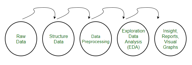
Steps in Data Preprocessing
Step 1: Import the necessary libraries
Python # importing libraries import pandas as pd import scipy import numpy as np from sklearn.preprocessing import MinMaxScaler import seaborn as sns import matplotlib.pyplot as plt
Step 2: Load the dataset
You can download dataset from here.
Python # Load the dataset df = pd.read_csv('Geeksforgeeks/Data/diabetes.csv') print(df.head()) Output:
Pregnancies Glucose BloodPressure SkinThickness Insulin BMI 0 6 148 72 35 0 33.6 \ 1 1 85 66 29 0 26.6 2 8 183 64 0 0 23.3 3 1 89 66 23 94 28.1 4 0 137 40 35 168 43.1 DiabetesPedigreeFunction Age Outcome 0 0.627 50 1 1 0.351 31 0 2 0.672 32 1 3 0.167 21 0 4 2.288 33 1
1. Check the data info
Python Output:
<class 'pandas.core.frame.DataFrame'> RangeIndex: 768 entries, 0 to 767 Data columns (total 9 columns): # Column Non-Null Count Dtype --- ------ -------------- ----- 0 Pregnancies 768 non-null int64 1 Glucose 768 non-null int64 2 BloodPressure 768 non-null int64 3 SkinThickness 768 non-null int64 4 Insulin 768 non-null int64 5 BMI 768 non-null float64 6 DiabetesPedigreeFunction 768 non-null float64 7 Age 768 non-null int64 8 Outcome 768 non-null int64 dtypes: float64(2), int64(7) memory usage: 54.1 KB
As we can see from the above info that the our dataset has 9 columns and each columns has 768 values. There is no Null values in the dataset.
We can also check the null values using df.isnull()
Python Output:
Pregnancies 0 Glucose 0 BloodPressure 0 SkinThickness 0 Insulin 0 BMI 0 DiabetesPedigreeFunction 0 Age 0 Outcome 0 dtype: int64
Step 2: Statistical Analysis
In statistical analysis we use df.describe() which will give a descriptive overview of the dataset.
Python Output:
.png) Data summary
Data summaryThe above table shows the count, mean, standard deviation, min, 25%, 50%, 75% and max values for each column. When we carefully observe the table we will find that Insulin, Pregnancies, BMI, BloodPressure columns has outliers.
Let's plot the boxplot for each column for easy understanding.
Step 3: Check the outliers
Python # Box Plots fig, axs = plt.subplots(9,1,dpi=95, figsize=(7,17)) i = 0 for col in df.columns: axs[i].boxplot(df[col], vert=False) axs[i].set_ylabel(col) i+=1 plt.show()
Output:
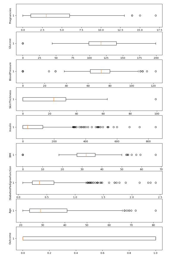 Boxplots
from the above boxplot we can clearly see that every column has some amounts of outliers.
Step 4: Drop the outliers
Python # Identify the quartiles q1, q3 = np.percentile(df['Insulin'], [25, 75]) # Calculate the interquartile range iqr = q3 - q1 # Calculate the lower and upper bounds lower_bound = q1 - (1.5 * iqr) upper_bound = q3 + (1.5 * iqr) # Drop the outliers clean_data = df[(df['Insulin'] >= lower_bound) & (df['Insulin'] <= upper_bound)] # Identify the quartiles q1, q3 = np.percentile(clean_data['Pregnancies'], [25, 75]) # Calculate the interquartile range iqr = q3 - q1 # Calculate the lower and upper bounds lower_bound = q1 - (1.5 * iqr) upper_bound = q3 + (1.5 * iqr) # Drop the outliers clean_data = clean_data[(clean_data['Pregnancies'] >= lower_bound) & (clean_data['Pregnancies'] <= upper_bound)] # Identify the quartiles q1, q3 = np.percentile(clean_data['Age'], [25, 75]) # Calculate the interquartile range iqr = q3 - q1 # Calculate the lower and upper bounds lower_bound = q1 - (1.5 * iqr) upper_bound = q3 + (1.5 * iqr) # Drop the outliers clean_data = clean_data[(clean_data['Age'] >= lower_bound) & (clean_data['Age'] <= upper_bound)] # Identify the quartiles q1, q3 = np.percentile(clean_data['Glucose'], [25, 75]) # Calculate the interquartile range iqr = q3 - q1 # Calculate the lower and upper bounds lower_bound = q1 - (1.5 * iqr) upper_bound = q3 + (1.5 * iqr) # Drop the outliers clean_data = clean_data[(clean_data['Glucose'] >= lower_bound) & (clean_data['Glucose'] <= upper_bound)] # Identify the quartiles q1, q3 = np.percentile(clean_data['BloodPressure'], [25, 75]) # Calculate the interquartile range iqr = q3 - q1 # Calculate the lower and upper bounds lower_bound = q1 - (0.75 * iqr) upper_bound = q3 + (0.75 * iqr) # Drop the outliers clean_data = clean_data[(clean_data['BloodPressure'] >= lower_bound) & (clean_data['BloodPressure'] <= upper_bound)] # Identify the quartiles q1, q3 = np.percentile(clean_data['BMI'], [25, 75]) # Calculate the interquartile range iqr = q3 - q1 # Calculate the lower and upper bounds lower_bound = q1 - (1.5 * iqr) upper_bound = q3 + (1.5 * iqr) # Drop the outliers clean_data = clean_data[(clean_data['BMI'] >= lower_bound) & (clean_data['BMI'] <= upper_bound)] # Identify the quartiles q1, q3 = np.percentile(clean_data['DiabetesPedigreeFunction'], [25, 75]) # Calculate the interquartile range iqr = q3 - q1 # Calculate the lower and upper bounds lower_bound = q1 - (1.5 * iqr) upper_bound = q3 + (1.5 * iqr) # Drop the outliers clean_data = clean_data[(clean_data['DiabetesPedigreeFunction'] >= lower_bound) & (clean_data['DiabetesPedigreeFunction'] <= upper_bound)]
Step 5: Correlation
Python #correlation corr = df.corr() plt.figure(dpi=130) sns.heatmap(df.corr(), annot=True, fmt= '.2f') plt.show()
Output:
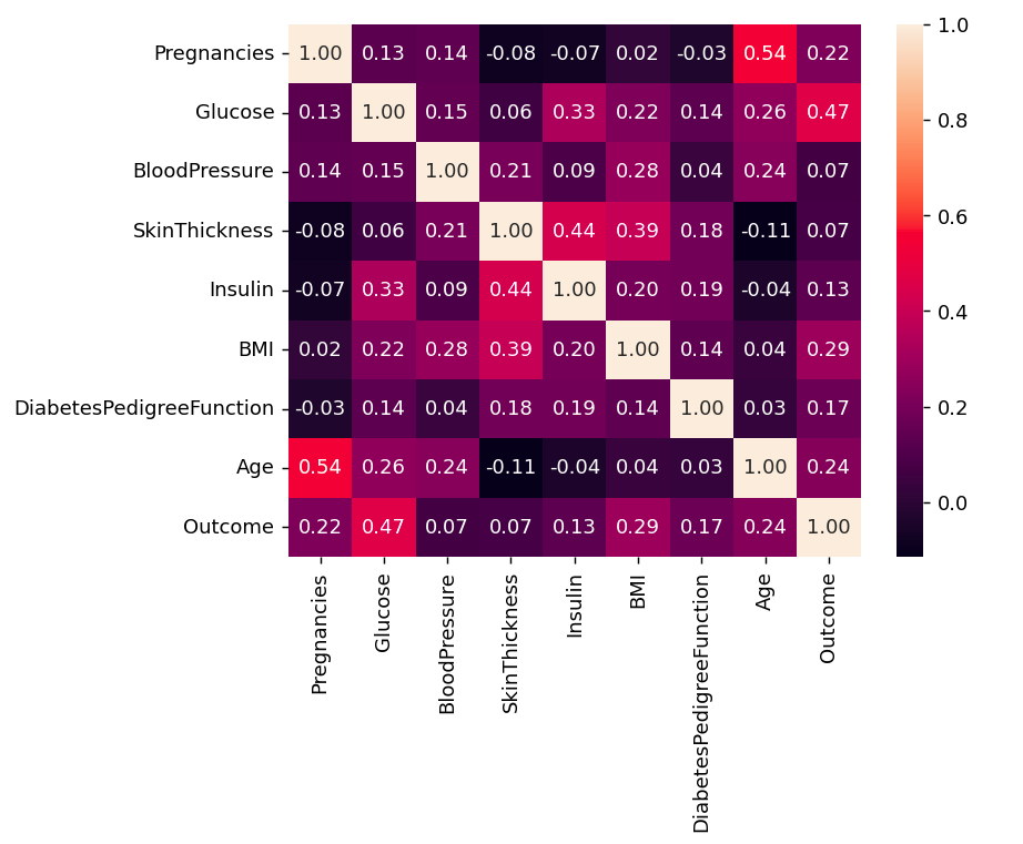 Correlation
We can also compare by single columns in descending order
Python corr['Outcome'].sort_values(ascending = False)
Output:
Outcome 1.000000 Glucose 0.466581 BMI 0.292695 Age 0.238356 Pregnancies 0.221898 DiabetesPedigreeFunction 0.173844 Insulin 0.130548 SkinThickness 0.074752 BloodPressure 0.0
Step 6: Check Outcomes Proportionality
Python plt.pie(df.Outcome.value_counts(), labels= ['Diabetes', 'Not Diabetes'], autopct='%.f', shadow=True) plt.title('Outcome Proportionality') plt.show() Output:
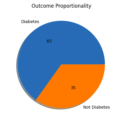 Outcome Proportionality
Step 7: Separate independent features and Target Variables
Python # separate array into input and output components X = df.drop(columns =['Outcome']) Y = df.Outcome
Step 7: Normalization or Standardization
Normalization
- Normalization works well when the features have different scales and the algorithm being used is sensitive to the scale of the features, such as k-nearest neighbors or neural networks.
- Rescale your data using scikit-learn using the MinMaxScaler.
- MinMaxScaler scales the data so that each feature is in the range [0, 1].
Python # initialising the MinMaxScaler scaler = MinMaxScaler(feature_range=(0, 1)) # learning the statistical parameters for each of the data and transforming rescaledX = scaler.fit_transform(X) rescaledX[:5]
Output:
array([[0.353, 0.744, 0.59 , 0.354, 0. , 0.501, 0.234, 0.483], [0.059, 0.427, 0.541, 0.293, 0. , 0.396, 0.117, 0.167], [0.471, 0.92 , 0.525, 0. , 0. , 0.347, 0.254, 0.183], [0.059, 0.447, 0.541, 0.232, 0.111, 0.419, 0.038, 0. ], [0. , 0.688, 0.328, 0.354, 0.199, 0.642, 0.944, 0.2 ]])
Standardization
- Standardization is a useful technique to transform attributes with a Gaussian distribution and differing means and standard deviations to a standard Gaussian distribution with a mean of 0 and a standard deviation of 1.
- We can standardize data using scikit-learn with the StandardScaler class.
- It works well when the features have a normal distribution or when the algorithm being used is not sensitive to the scale of the features
Python from sklearn.preprocessing import StandardScaler scaler = StandardScaler().fit(X) rescaledX = scaler.transform(X) rescaledX[:5]
Output:
array([[ 0.64 , 0.848, 0.15 , 0.907, -0.693, 0.204, 0.468, 1.426], [-0.845, -1.123, -0.161, 0.531, -0.693, -0.684, -0.365, -0.191], [ 1.234, 1.944, -0.264, -1.288, -0.693, -1.103, 0.604, -0.106], [-0.845, -0.998, -0.161, 0.155, 0.123, -0.494, -0.921, -1.042], [-1.142, 0.504, -1.505, 0.907, 0.766, 1.41 , 5.485]
In conclusion data preprocessing is an important step to make raw data clean for analysis. Using Python we can handle missing values, organize data and prepare it for accurate results. This ensures our model is reliable and helps us uncover valuable insights from data.
Similar Reads
Machine Learning Tutorial Machine learning is a branch of Artificial Intelligence that focuses on developing models and algorithms that let computers learn from data without being explicitly programmed for every task. In simple words, ML teaches the systems to think and understand like humans by learning from the data.Machin
5 min read
Introduction to Machine Learning
Python for Machine Learning
Machine Learning with Python TutorialPython language is widely used in Machine Learning because it provides libraries like NumPy, Pandas, Scikit-learn, TensorFlow, and Keras. These libraries offer tools and functions essential for data manipulation, analysis, and building machine learning models. It is well-known for its readability an
5 min read
Pandas TutorialPandas is an open-source software library designed for data manipulation and analysis. It provides data structures like series and DataFrames to easily clean, transform and analyze large datasets and integrates with other Python libraries, such as NumPy and Matplotlib. It offers functions for data t
6 min read
NumPy Tutorial - Python LibraryNumPy (short for Numerical Python ) is one of the most fundamental libraries in Python for scientific computing. It provides support for large, multi-dimensional arrays and matrices along with a collection of mathematical functions to operate on arrays.At its core it introduces the ndarray (n-dimens
3 min read
Scikit Learn TutorialScikit-learn (also known as sklearn) is a widely-used open-source Python library for machine learning. It builds on other scientific libraries like NumPy, SciPy and Matplotlib to provide efficient tools for predictive data analysis and data mining.It offers a consistent and simple interface for a ra
3 min read
ML | Data Preprocessing in PythonData preprocessing is a important step in the data science transforming raw data into a clean structured format for analysis. It involves tasks like handling missing values, normalizing data and encoding variables. Mastering preprocessing in Python ensures reliable insights for accurate predictions
6 min read
EDA - Exploratory Data Analysis in PythonExploratory Data Analysis (EDA) is a important step in data analysis which focuses on understanding patterns, trends and relationships through statistical tools and visualizations. Python offers various libraries like pandas, numPy, matplotlib, seaborn and plotly which enables effective exploration
6 min read
Feature Engineering
Supervised Learning
Unsupervised Learning
Model Evaluation and Tuning
Advance Machine Learning Technique
Machine Learning Practice