We capture the world with cameras that compress depth, texture, and geometry into flat pixel grids, yet our minds effortlessly reconstruct the 3D structure behind them. What if computers could do the same? Structure-from-Motion (SfM) is the technique that enables this. By analyzing how features shift across multiple images, SfM simultaneously recovers the camera motion and the scene’s underlying 3D shape, effectively “lifting” depth from 2D photographs.

In this post, we’ll explore SfM theory, its pipeline, and a hands-on C++ tutorial using OpenCV’s SfM module to perform 3D scene reconstruction, recover camera poses, and generate a sparse 3D point cloud from a set of images. Whether you’re curious about photogrammetry or 3D reconstruction, this guide takes you from concepts to a working application.

1. What Is Structure from Motion (SfM)?

Structure from Motion (SfM) is a technique that reconstructs 3D structure (points in space) and estimates camera motion (poses and sometimes intrinsics) using only a sequence of 2D images captured from different viewpoints. In other words, SfM takes ordinary photographs and infers both where the camera moved and what the scene looks like in 3D. It requires no depth sensors, no GPS, and no manual annotation, making it a widely used unsupervised method for 3D reconstruction.

1.1. What Is the OpenCV SfM Module?

The OpenCV SfM module (cv::sfm) is OpenCV’s implementation of the classical Structure from Motion pipeline.

The module provides a high-level interface that automatically performs the complete SfM workflow internally, including feature extraction, matching, pose estimation, triangulation, and global bundle adjustment. Internally, OpenCV SfM is built on top of the libmv multi-view geometry library and uses the Ceres Solver for non-linear optimization.

Instead of exposing every low-level SfM step to the user, OpenCV simplifies the workflow through a single primary function:

cv::sfm::reconstruct(...)

This function internally performs feature matching, pose estimation, triangulation, and bundle adjustment, and directly returns:

• The estimated camera rotation matrices
• The estimated camera translation vectors
• A sparse 3D point cloud of the scene

1.2. What is the use of SfM, and how is it useful?

Although SfM produces only a sparse 3D representation, it is one of the most widely used techniques in modern 3D vision systems because it accurately recovers camera motion and reliable geometric structure. These outputs underpin many real-world computer vision applications.

Applications of Structure from Motion (SfM):

1. Robotics and Autonomous Navigation: SfM is used to estimate camera motion and build sparse maps for robot and drone localization and navigation.
2. Augmented Reality (AR): SfM enables real-time camera tracking and stable placement of virtual objects in real-world scenes.
3. Photogrammetry and Drone Mapping: SfM is the first stage in generating 3D maps and models from aerial or ground-based images.
4. Visual Effects (VFX) and Camera Tracking: SfM is used to recover real camera motion so that CGI elements can be accurately inserted into videos.
5. 3D Vision Research and System Evaluation: SfM is widely used to evaluate feature matching, camera calibration, and multi-view geometry algorithms.
6. Foundation for Dense 3D Reconstruction: SfM provides camera poses and geometric constraints required for dense reconstruction using Multi-View Stereo.

2. Overview of the SfM Pipeline

Structure-from-motion sounds complex, but it always boils down to the same sequence of steps. In this section, we will walk through the pipeline conceptually. In the next section, we will map each step of the actual C++ code used for 3D Scene reconstruction.

A typical SfM pipeline includes:

1. Data Collection and Image List
2. Camera Instrincs and Calibration
3. Feature Detection and Matching
4. Incremental reconstruction and camera poses
5. Triangulation and sparse 3D point cloud
6. Bundle adjustment and refinement

2.1. Data Collection and Image List

The first step is to gather a set of images that adequately cover the scene or object you want to reconstruct. Some important considerations:

• Overlapping views: Consecutive images must share sufficient common features to enable matching.
• Varied perspectives: Different angles provide depth cues and parallax, essential for accurate reconstruction.
• Consistent lighting: While SfM can tolerate moderate lighting changes, extreme variations may reduce feature matching accuracy.

Once collected, the image paths are stored in a text file (.txt) that the SfM pipeline reads sequentially. This list informs the algorithm which images to process and in what order.

2.2. Camera Instrinsics and Calibration

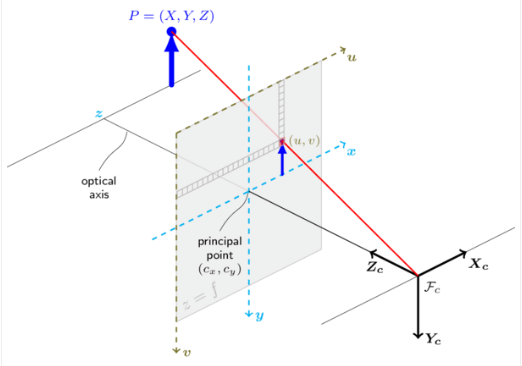
Before we can reason about 3D geometry, we need to understand how a camera projects 3D points onto a 2D image plane. The camera intrinsic matrix, K, captures this relationship:

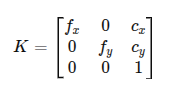
Here, fx and fy are the focal lengths of the camera projection expressed in pixels units along the x and y axes, while cx and cy represent the coordinates of the principal point, usually located near the center of the image.

There are two main ways to obtain these intrinsics:

1. Calibrated camera – The most accurate approach is to perform a camera calibration using a checkerboard or calibration target (e.g., OpenCV’s calibrateCamera). This procedure yields precise values for fx, fy, cx, cy, resulting in more reliable 3D reconstructions.

2. Approximate intrinsics – When calibration is unavailable, a reasonable approximation can be derived from the image size. A common approach is to:

• Set the focal length proportional to the image width.
• Assume the principal point lies at the image center.

For example, in the provided code:

 f  = 0.9 * static_cast<double>(width); cx = width  * 0.5; cy = height * 0.5; Matx33d K(f, 0, cx,           0, f, cy,           0, 0, 1); 

Note: This approximation does not provide a metric scale but offers a good starting point for the SfM solver.

The intrinsic matrix is a key ingredient in the SfM pipeline. It is used to:

• Convert pixel coordinates into rays in camera space
• Relate 2D observations to 3D points
• Stabilize camera pose estimation and triangulation

In short, accurate intrinsics lead to better camera poses, which directly improve the quality of the reconstructed 3D scene.

2.3. Feature Detection and Matching

SfM relies on correspondence, identifying which pixels in different images represent the same 3D point. This step is crucial because everything that follows depends on accurate matches.

The process has two main stages:

• Feature detection: Algorithms like SIFT (Scale-Invariant Feature Transform) or ORB scan the image for “keypoints”, distinctive areas like corners or blobs that are recognizable even if the image is scaled or rotated.
• Feature description and matching: Each keypoint is assigned a descriptor based on the pixel-intensity patterns around it. We compare these descriptors between Image A and Image B. If the descriptors match, we assume they refer to the same physical point. 

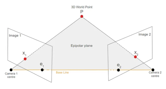
Geometric Verification (RANSAC): Many matches will be incorrect (e.g., a window on one building may appear to be a window on another). We use RANSAC (Random Sample Consensus) to find the Fundamental Matrix (F) or Essential Matrix (E), effectively filtering out matches that don’t obey the laws of geometry.

The Fundamental Matrix (F) encodes the epipolar geometry between two uncalibrated camera views, relating corresponding points across images. The Essential Matrix (E) represents the same geometric relationship but for calibrated cameras, and it is used to recover the relative camera rotation and translation.

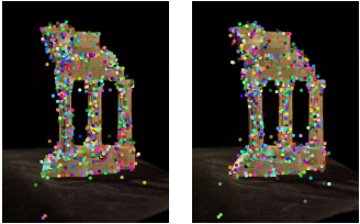
Fig 2: Feature extraction performed in the two images 

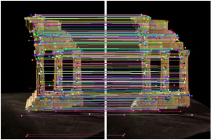
Fig 3: Feature matching between the two images

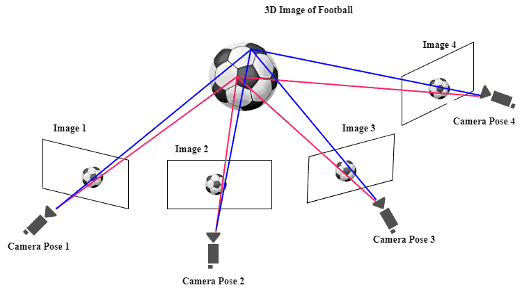
2.4. Incremental reconstruction and camera poses

Once we have feature correspondences, the next step is to estimate each camera’s position at the time it captured its image.

1. Initialization: Pick two images with good overlap and a wide baseline (distance between them).
2. Pose Estimation: Decompose the Essential Matrix (E) to find the Rotation (R) and Translation (t) of the second camera relative to the first.
3. PnP (Perspective-n-Point): As we add a third image, we identify features in the new image that correspond to 3D points we have already found. We use these known 3D-2D correspondences to calculate the pose of the new camera.

2.5. Triangulation and sparse 3D point cloud

With camera poses and 2D feature matches available, we can now triangulate 3D points. 

• A 3D point appears in multiple images, giving different pixel locations, and each pixel defines a 3D ray from the camera center into the scene.
• Intersection: ideally, these rays meet at a single point in 3D space.
• Approximation: Due to noise, they rarely intersect perfectly, so we compute the 3D point that best fits all rays (least-squares solution).
• Sparse cloud: doing this for all feature tracks yields a sparse point cloud composed of meaningful scene points (corners, edges, textured areas), while flat or textureless regions contribute few points.
• Result: this sparse cloud represents the reconstructed scene and serves as the geometric foundation for further refinement or dense reconstruction. In OpenCV, these points are returned as points3d_estimated and can be exported (e.g., PLY) for visualization tools such as MeshLab or CloudCompare.

2.6. Bundle adjustment and refinement

This is the “optimization” layer. As we add more cameras, minor errors accumulate (drift). The reconstruction might start to bend or curve unnaturally.

• The Goal: Minimize the reprojection error (the difference between the predicted pixel position of a 3D point and the actual detected feature).
• The Process: Bundle adjustment jointly refines all camera poses (Ri, ti) and 3D points Xj​. Each point is reprojected into the images where it appears, and these predicted locations are compared with the actual keypoints. The solver then adjusts all poses and points together to minimize the overall reprojection error.
• The Optimization: This forms a large non-linear least-squares problem. Solving it sharpens the camera trajectory, pulls 3D points into more accurate locations, and suppresses unstable or inconsistent points, resulting in a clean and coherent reconstruction.
• In OpenCV:
  • Bundle adjustment is handled internally using Ceres Solver.
  • Calling cv::sfm::reconstruct() automatically returns optimized poses and 3D points.

2.7. The cv::sfm::reconstruct API in OpenCV

The cv::sfm::reconstruct function provides a high-level interface to the entire Structure-from-Motion pipeline.

5K+ Learners
3 Hours of Learning

Join Free VLM Bootcamp

100K+ Learners
3 Hours of Learning

Join Free OpenCV Bootcamp

15K+ Learners
3 Hours of Learning

Join Free TensorFlow Bootcamp

10K+ Learners
8 Hours of Learning

Join Free PyTorch Bootcamp

View all AI Free Courses

This single API call executes the complete SfM workflow internally, including feature extraction, feature matching, incremental camera pose estimation, triangulation, and global bundle adjustment. It is designed to abstract away the low-level multi-view geometry steps, allowing users to focus on inputs and outputs.

Here is the essential breakdown of the API based code:

 cv::sfm::reconstruct(     imagePaths, //  Input: List of image files     Rs,         //  Output: Camera Rotations (poses)     ts,         //  Output: Camera Translations (poses)     K,          //  Input/Output: Camera Intrinsics (f, cx, cy)     points3d,   //  Output: The 3D Sparse Point Cloud     isProjective//   Input: Optimization flag ); 

What Happens Inside:  

Calling this API triggers the whole sequence described in the pipeline:

1. Feature Matching: Finds and verifies corresponding keypoints across all images.
2. Initial Pose: Determines the starting position of the first few cameras.
3. Triangulation: Converts matched 2D points into initial 3D points.
4. Bundle Adjustment: Runs a large-scale, non-linear optimization (using Ceres) to simultaneously refine all camera poses and all 3D points, minimizing all accumulated errors.

3. 3D Scene Reconstruction Using OpenCV SfM

Having understood the conceptual pipeline, we now map it to a C++ implementation using the OpenCV SfM module. The sfm_reconstruction.cpp program demonstrates how to perform end-to-end 3D scene reconstruction from a list of images with just a few dozen lines of code.

Dataset: TempleRing

For this reconstruction, we use the TempleRing dataset, a standard benchmark for multi-view geometry and 3D reconstruction. It contains about images at a 640 × 480 resolution with known camera intrinsics and substantial viewpoint overlap. These properties make it well-suited for validating the accuracy and stability of the SfM pipeline.

Step 1: Setup and Dependencies

Before building and running the program, the following are required:

• OpenCV with opencv_contrib, including the sfm and viz modules
• Ceres Solver for bundle adjustment
• A C++17 compatible compiler (e.g., g++)

The project is built using CMake. The provided CMakeLists.txt:

• Sets the C++17 standard
• Finds the required OpenCV modules (core, highgui, viz, sfm)
• Links them to the sfm_reconstruction executable and enables Ceres support

Once these dependencies are available, the project can be built using the standard CMake workflow.

Step 2: The Implementation

This program takes a list of images and camera parameters, runs the reconstruction, and saves the result as a .ply file for visualization.

sfm_reconstruction.cpp 

 int main(int argc, char** argv) { if (argc != 5) { cout << "Usage: " << argv[0] << " image_paths.txt f cx cy\n"; return 0; } // 1. Load input image list string listFile = argv[1]; vector<String> imagePaths; if (!loadImageList(listFile, imagePaths)) { cerr << "Failed to load image list.\n"; return -1; } cout << "[INFO] Loaded " << imagePaths.size() << " images.\n"; // 2. Read camera intrinsics from command line double f = atof(argv[2]); double cx = atof(argv[3]); double cy = atof(argv[4]); Matx33d K(f, 0, cx, 0, f, cy, 0, 0, 1); cout << "[INFO] Camera Intrinsics K:\n" << Mat(K) << endl; // 3. Run the OpenCV SfM pipeline bool isProjective = true; // Projective reconstruction vector<Mat> Rs, ts, points3d; cout << "[INFO] Running SfM reconstruction...\n"; cv::sfm::reconstruct(imagePaths, Rs, ts, K, points3d, isProjective); // 4. Output basic reconstruction statistics cout << "[INFO] Reconstruction complete.\n"; cout << "Estimated cameras: " << Rs.size() << endl; cout << "Reconstructed 3D points: " << points3d.size() << endl; return 0; } 

( The complete working source code for this example is available on this blog )

CmakeLists.txt

 cmake_minimum_required(VERSION 3.10) project(sfm_reconstruction) set(CMAKE_CXX_STANDARD 17) set(CMAKE_CXX_STANDARD_REQUIRED ON) # Adjust this if your OpenCV is in a different place set(OpenCV_DIR /usr/local/lib/cmake/opencv4) find_package(OpenCV REQUIRED sfm viz highgui core) include_directories(/usr/local/include/opencv4) add_executable(sfm_reconstruction sfm_reconstruction.cpp) target_link_libraries(sfm_reconstruction ${OpenCV_LIBS}) target_compile_definitions(sfm_reconstruction PRIVATE CERES_FOUND=1) 

3.1. How to Run the SfM Example

1. Prepare the image list: Create image_paths.txt with paths to all images, one per line.
2. Build the project: Run cmake and then execute the below-mentioned command on the terminal,
   • make -j$(nproc)
3. Run the program using the command:
   • ./build/sfm_reconstruction image_paths.txt 800 400 225

The numbers set the camera intrinsics (f, cx, cy). Here, 800 is the focal length, and 400 and 225 are the principal point coordinates (cx, cy) in pixels. If these values are omitted, the program automatically estimates them from the image size.

How This Implementation Maps to the SfM Pipeline

Each step of the theoretical SfM pipeline discussed earlier directly corresponds to a component of this implementation:

• Data collection and image list → Image paths loaded from the text file
• Camera intrinsics and calibration → Intrinsic matrix K estimated from image size
• Feature detection and matching → Handled internally by cv::sfm::reconstruct()
• Incremental reconstruction and camera poses → Output as Rs_est and ts_est
• Triangulation and sparse point cloud → Output as points3d_estimated
• Bundle adjustment and refinement → Performed internally using Ceres Solver

Thus, sfm_reconstruction.cpp serves as a compact, end-to-end demonstration of the full SfM pipeline, from raw images to a sparse 3D reconstruction and camera trajectory.

3.2. Output and Visualization:

The reconstruction output consists of a sparse 3D point cloud shown as green points and the estimated camera trajectory visualized using yellow lines and white camera frustums in Fig 6 below. The point cloud represents only reliable feature-based landmarks and not a complete surface, which is the expected behavior of a sparse SfM pipeline. Even with fewer points, the output correctly captures the 3D structure of the scene and the camera motion.

Visualization:

OpenCV Viz window displaying the camera path and sparse point cloud

Point cloud in MeshLab using the exported .ply file

Color Coding:

• Green → Sparse 3D structure
• Yellow → Camera trajectory
• White → Camera frustums

The above result represents a sparse 3D reconstruction, not a dense mesh or surface model. It serves as the geometric foundation for further dense reconstruction or vision-based applications.

4. Conclusion

Structure-from-Motion is a powerful technique that enables true 3D understanding from ordinary 2D images. In this article, we explored how the SfM pipeline works, how it is implemented in OpenCV, and how it can be used to build a complete end-to-end 3D scene reconstruction system. We visualized the recovered camera poses and the sparse 3D point cloud, and exported the results for use with external tools such as MeshLab.

OpenCV’s SfM module provides an excellent entry point into multi-view geometry, 3D vision, robotics, and photogrammetry, making it especially valuable for learning, research, and rapid prototyping.

REFERENCES:

3D Reconstruction via Incremental Structure From Motion – Paper

Structure from Motion – OpenCV documentation