I've been working on the following polynomial approximation problem. I want to find the optimal Chebyshev approximation of the rational function $\frac{1}{1-x}$ on the real interval $x\in[-\rho, \rho]$, $\rho<1$ using $T$-degree polynomials $h_T(x)$. I formulate the approximation problem as the following optimization problem: $$ \min_{\alpha_i} \left\|\frac{1}{1-x}-\alpha_Tx^T-\alpha_{T-1}x^{T-1}-\cdots-\alpha_1x-\alpha_0\right\|_{\infty, \rho}, $$ where the notation $\lVert\cdot\rVert_{\infty, \rho}$ stands for the Chebyshev norm of polynomials defined as: $$ \lVert f(x)\rVert_{\infty, \rho}=\sup_{x\in[-\rho, \rho]} \lvert f(x)\rvert. $$ Currently, I can solve the above problem numerically using the Pólya–Szegő theorem. To be specific, the above optimization problem can be massaged as: $$ \begin{aligned} & \min_{\alpha_i}\ \delta, \\ s.t.\ & \frac{1}{1-x}-\sum_{i=0}^T\alpha_ix^i\leq \delta, \forall x\in[-\rho, \rho], \\ & \frac{1}{1-x}-\sum_{i=0}^T \alpha_ix^i\geq -\delta, \forall x\in[-\rho, \rho], \end{aligned} $$$$ \begin{aligned} & \min_{\alpha_i}\ \delta, \\ \text{s.t. } & \frac{1}{1-x}-\sum_{i=0}^T\alpha_ix^i\leq \delta, \forall x\in[-\rho, \rho], \\ & \frac{1}{1-x}-\sum_{i=0}^T \alpha_ix^i\geq -\delta, \forall x\in[-\rho, \rho], \end{aligned} $$ which could be further modified to: $$ \begin{aligned} & \min_{\alpha_i}\ \delta, \\ s.t.\ & -1+(1-x)\left(\sum_{i=0}^T\alpha_ix^i+\delta\right)\geq 0, \forall x\in[-\rho, \rho], \\ & 1+(1-x)\left(-\sum_{i=0}^T \alpha_ix^i+\delta\right)\geq 0, \forall x\in[-\rho, \rho]. \end{aligned} $$ According to Powers and Reznick - Polynomials that are positive on an interval, the inequalities of the optimization problem hold as long as the polynomials on the LHS can be written as $(f(x))^2+(\rho^2-x^2)(g(x))^2$, where $f(x)$ is a $T$-degree polynomial and $g(x)$ is a ($T-1$)-degree polynomial.
Using this technique, I massaged the above optimization problem in the polynomial form to an equivalent Semi-Definite Programming (SDP) problem and solved the problem using SDP solvers.
Here are some numerical results I've got so far. First, I observe that the approximation error decreases exponentially w.r.t. the degree of the polynomial $h_T(x)$, and my simulation result is 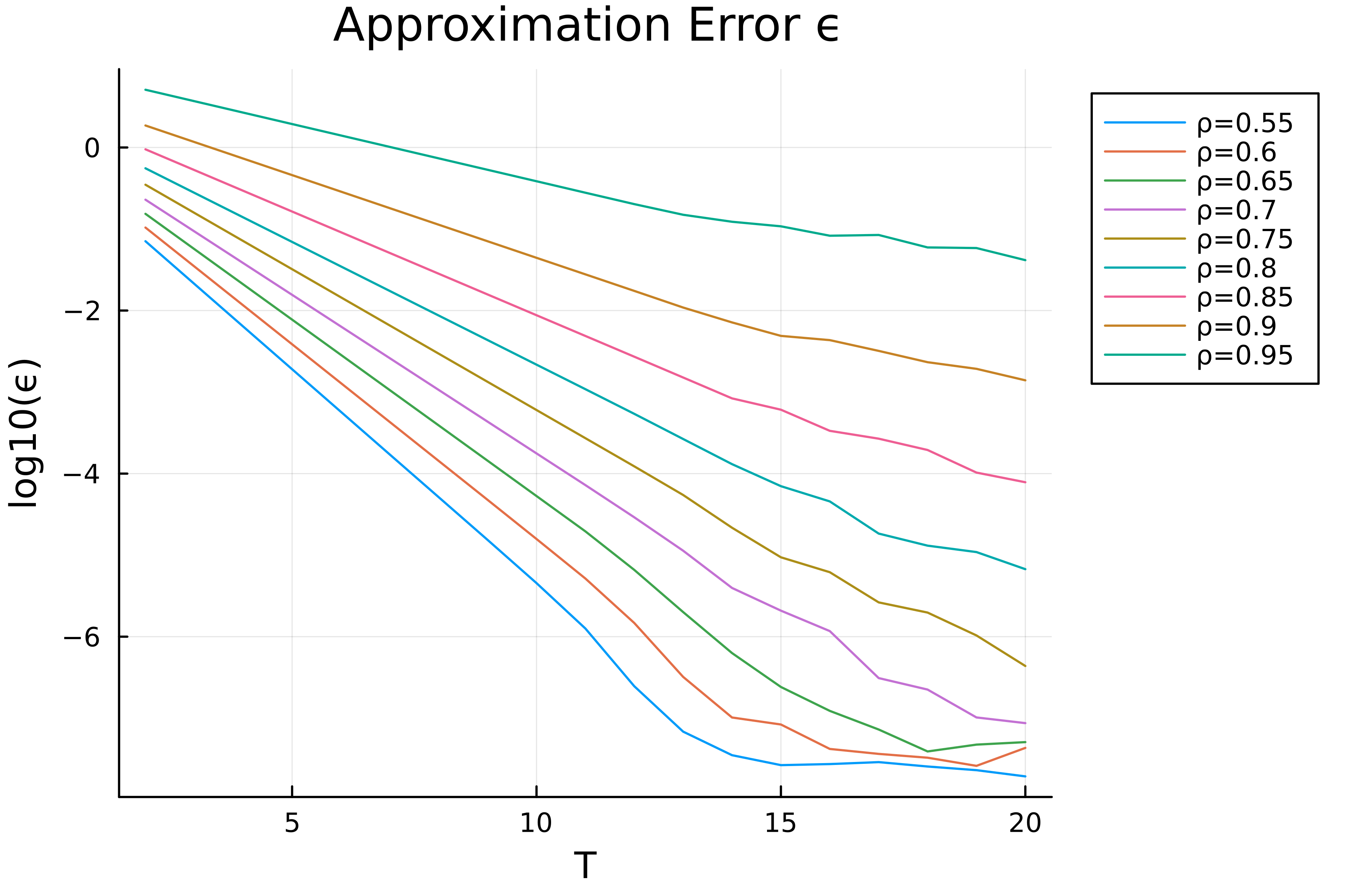 It can be seen that the approximation error attenuates exponentially w.r.t. $T$ before $T=12$. I believe that my SDP solver may suffer from numerical issues when the approximation error $\epsilon\leq 1e-7$ (maybe because I set the duality gap of the solver to be $1e-6$) or when the dimension of the matrices are large so that the curve looks weird after $T=12$.
Moreover, I study the relationship between the approximation error and the length of the interval $\rho$ plotted here 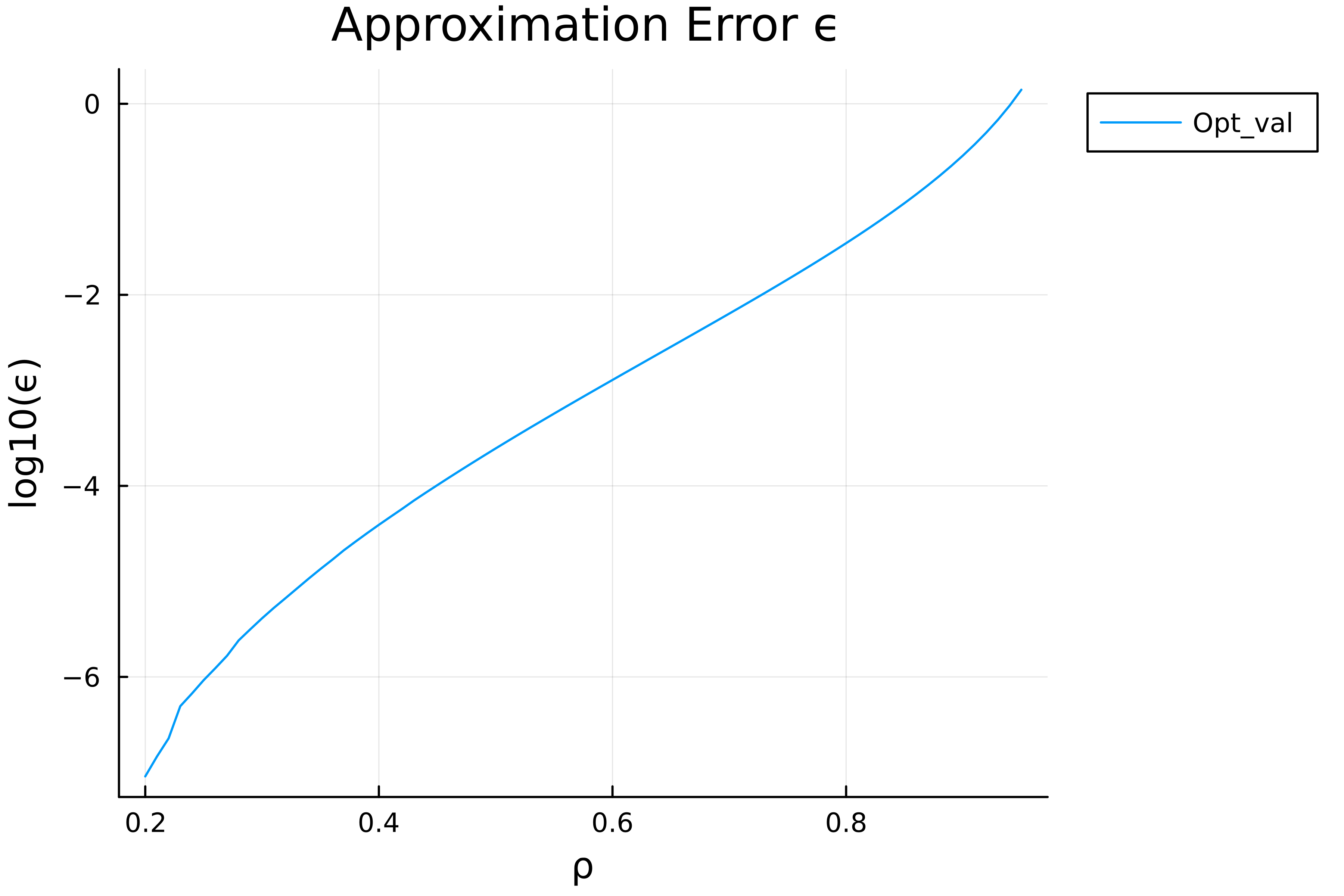 (the degree of $h_T(x)$ is fixed to be $T=6$). It seems that the relationship is approximately (but not exactly) exponential.
On the other hand, I am also interested in the magnitude of the coefficients $\lVert\boldsymbol{\alpha}\rVert_1$, where $\boldsymbol{\alpha}=\left[\alpha_0, \alpha_1, \dotsc, \alpha_T\right]$. The magnitude $\lVert\boldsymbol{\alpha}\rVert_1$ w.r.t. $T$ are visualized in 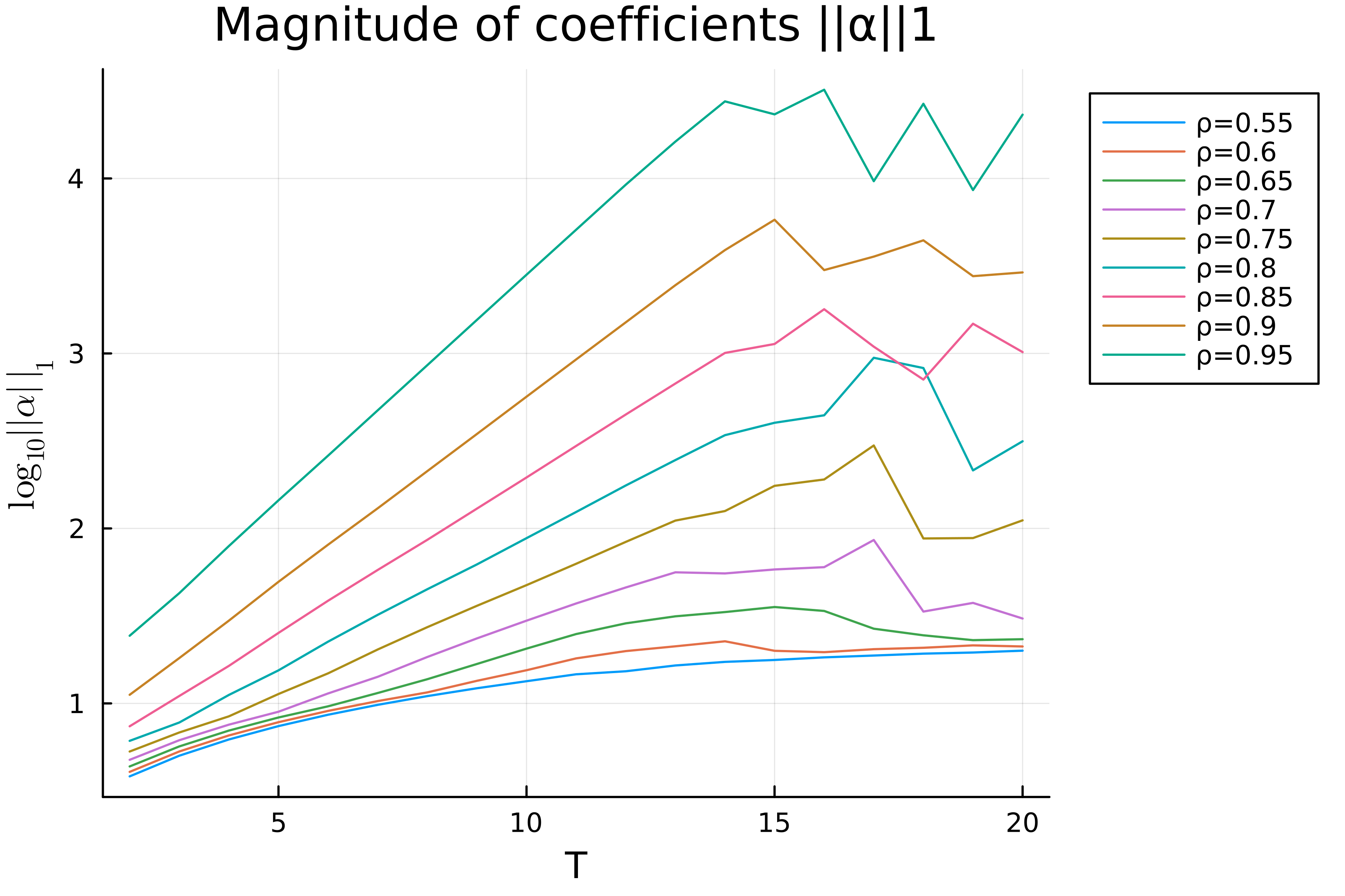 and $\lVert\boldsymbol{\alpha}\rVert_1$ w.r.t. $\rho$ here
 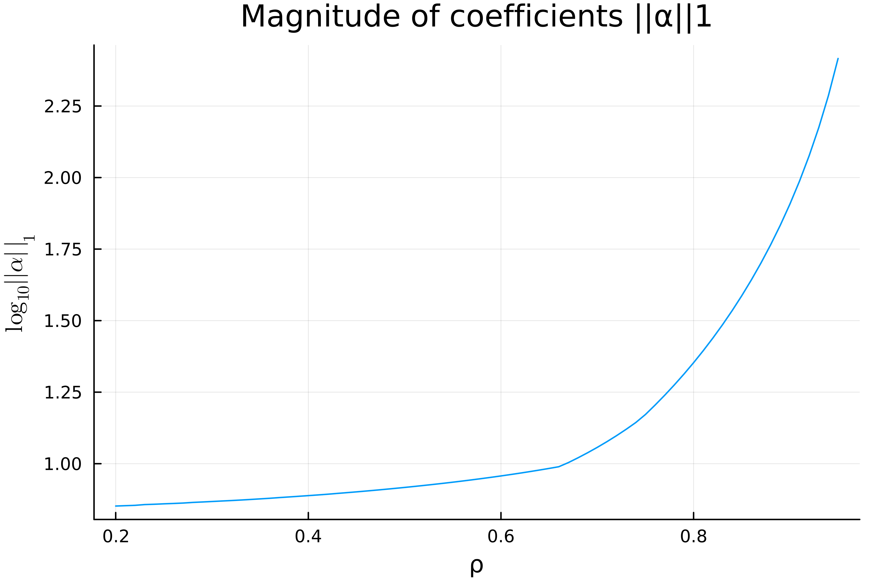 (still $T=6$). It can be seen that $\lVert\boldsymbol{\alpha}\rVert_1$ grows linearly with $T$ for a small $\rho$, and grows exponentially w.r.t. $T$ for a large $\rho$ ($\rho\geq 0.7$). Besides, $\lVert\boldsymbol{\alpha}\rVert_1$ increases quicker than exponentially w.r.t. $\rho$.
Despite the numerical results so far, the problem lacks theoretical guarantee on both the approximation error $\epsilon$ and the magnitude of the coefficients $\lVert\boldsymbol{\alpha}\rVert_1$. Could anyone help me to find a way out?