(Note that mind-map’s PDF has hyperlinks. Also, see the folder Presentation-aids. )
Approximately 70% of the presentation was based on an R-programmed software monad for epidemiology compartmental models, ECMMon-R, [AAr2]. For the rest were used frameworks, simulations, and graphics made with Mathematica, [AAr1], and Wolfram System Modeler .
The presentation was given online (because of COVID-19) using Zoom. 190 people registered. Nearly 70 showed up (and maybe 60 stayed throughout.)
“SEI2HR” stands for “Susceptible, Exposed, Infected two, Hospitalized, Recovered” (populations.) “Econ” stands for “Economic”.
In this notebook we also deal with both quarantine scenarios and medical supplies scenarios. In the notebook [AA4] we deal with quarantine scenarios over a simpler model, SEI2HR.
Remark: We consider the contagious disease propagation models as instances of the more general System Dynamics (SD) models. We use SD terminology in this notebook.
The models
SEI2R
The model SEI2R is introduced and explained in the notebook [AA2]. SEI2R differs from the classical SEIR model, [Wk1, HH1], with the following elements:
Two separate infected populations: one is “severely symptomatic”, the other is “normally symptomatic”
The monetary equivalent of lost productivity due to infected or died people is tracked
SEI2HR
For the formulation of SEI2HR we use a system of Differential Algebraic Equations (DAE’s). The package [AAp1] allows the use of a formulation that has just Ordinary Differential Equations (ODE’s).
Here are the unique features of SEI2HR:
People stocks
There are two types of infected populations: normally symptomatic and severely symptomatic.
There is a hospitalized population.
There is a deceased from infection population.
Hospital beds
Hospital beds are a limited resource that determines the number of hospitalized people.
Only severely symptomatic people are hospitalized according to the available hospital beds.
The hospital beds stock is not assumed constant, it has its own change rate.
Money stocks
The money from lost productivity is tracked.
The money for hospital services is tracked.
SEI2HR-Econ
SEI2HR-Econ adds the following features to SEI2HR:
Medical supplies
Medical supplies production is part of the model.
Medical supplies delivery is part of the model..
Medical supplies accumulation at hospitals is taken into account.
Medical supplies demand tracking.
Hospitalization
Severely symptomatic people are hospitalized according to two limited resources: hospital beds and medical supplies.
Money stocks
Money for medical supplies production is tracked.
SEI2HR-Econ’s place a development plan
This graph shows the “big picture” of the model development plan undertaken in [AAr1] and SEI2HR (discussed in this notebook) is in that graph:
Notebook structure
The rest of notebook has the following sequence of sections:
Package load section
SEI2HR-Econ structure in comparison of SEI2HR
Explanations of the equations of SEI2HR-Econ
Quarantine scenario modeling preparation
Medical supplies production and delivery scenario modeling preparation
Parameters and initial conditions setup
Populations, hospital beds, quarantine scenarios, medical supplies scenarios
Simulation solutions
Interactive interface
Sensitivity analysis
Load packages
The epidemiological models framework used in this notebook is implemented with the packages [AAp1-AAp4, AA3]; many of the plot functions are from the package [AAp5].
In this section we provide rationale for the equations of SEI2HR-Econ.
The equations for Susceptible, Exposed, Infected, Recovered populations of SEI2R are “standard” and explanations about them are found in [WK1, HH1]. For SEI2HR those equations change because of the stocks Hospitalized Population and Hospital Beds. For SEI2HR-Econ the SEI2HR equations change because of the stocks Medical Supplies, Medical Supplies Demand, and Hospital Medical Supplies.
The equations time unit is one day. The time horizon is one year. Since we target COVID-19, [Wk2, AA1], we do not consider births.
Remark: For convenient reading the equations in this section have tooltips for the involved stocks and rates.
Verbalization description of the model
We start with one infected (normally symptomatic) person, the rest of the people are susceptible. The infected people meet other people directly or get in contact with them indirectly. (Say, susceptible people touch things touched by infected.) For each susceptible person there is a probability to get the decease. The decease has an incubation period: before becoming infected the susceptible are (merely) exposed. The infected recover after a certain average infection period or die. A certain fraction of the infected become severely symptomatic. The severely symptomatic infected are hospitalized if there are enough hospital beds and enough medical supplies. The hospitalized severely infected have different death rate than the non-hospitalized ones. The number of hospital beds might change: hospitals are extended, new hospitals are build, or there are not enough medical personnel or supplies.
The different types of populations (infected, hospitalized, recovered, etc.) have their own consumption rates of medical supplies. The medical supplies are produced with a certain rate (units per day) and delivered after a certain delay period. The hospitals have their own storage for medical supplies. Medical supplies are delivered to the hospitals only, non-hospitalized people go to the medical supplies producer to buy supplies. The hospitals have precedence for the medical supplies: if the medical supplies are not enough for everyone, the hospital needs are covered first (as much as possible.)
The medical supplies producer has a certain storage capacity (for supplies.) The medical supplies delivery vehicles have a certain – generally speaking, smaller – capacity. The hospitals have a certain capacity to store medical supplies. It is assumed that both producer and hospitals have initial stocks of medical supplies. (Following a certain normal, general preparedness protocol.)
The combined demand from all populations for medical supplies is tracked (accumulated.) The deaths from infection are tracked (accumulated.) Money for medical supplies production, money for hospital services, and money from lost productivity are tracked (accumulated.)
The equations below give mathematical interpretation of the model description above.
Code for the equations
Each equation in this section are derived with code like this:
and then the output cell is edited to be “DisplayFormula” and have CellLabel value corresponding to the stock of interest.
The infected and hospitalized populations
SEI2HR has two types of infected populations: a normally symptomatic one and a severely symptomatic one. A major assumption for SEI2HR is that only the severely symptomatic people are hospitalized. (That assumption is also reflected in the diagram in the introduction.)
Each of those three populations have their own contact rates and mortality rates.
Here are the contact rates from the SEI2HR-Econ dictionary
Remark: Below with “Infected Population” we mean both stocks Infected Normally Symptomatic Population (INSP) and Infected Severely Symptomatic Population (ISSP).
Total Population
In this notebook we consider a DAE’s formulation of SEI2HR-Econ. The stock Total Population has the following (obvious) algebraic equation:
0z7878rbvh3ut
Note that with Max we specified that the total population cannot be less than .
Remark: As mentioned in the introduction, the package [AAp1] allows for the use of non-algebraic formulation, without an equation for TP.
Susceptible Population
The stock Susceptible Population (SP) is decreased by (1) infections derived from stocks Infected Populations and Hospitalized Population (HP), and (2) morality cases derived with the typical mortality rate.
1gercwr5szizt
Because we hospitalize the severely infected people only instead of the term
09xmdu8xq7e0p
we have the terms
0dkc6td55qv7p
The first term is for the infections derived from the hospitalized population. The second term for the infections derived from people who are infected severely symptomatic and not hospitalized.
Births term
Note that we do not consider in this notebook births, but the births term can be included in SP’s equation:
The births rate is the same as the death rate, but it can be programmatically changed. (See [AAp2].)
Exposed Population
The stock Exposed Population (EP) is increased by (1) infections derived from the stocks Infected Populations and Hospitalized Population, and (2) mortality cases derived with the typical mortality rate. EP is decreased by (1) the people who after a certain average incubation period (aincp) become ill, and (2) mortality cases derived with the typical mortality rate.
083x1htqp0kkx
Infected Normally Symptomatic Population
INSP is increased by a fraction of the people who have been exposed. That fraction is derived with the parameter severely symptomatic population fraction (sspf). INSP is decreased by (1) the people who recover after a certain average infection period (aip), and (2) the normally symptomatic people who die from the disease.
01cfzpu1jv3o4
Infected Severely Symptomatic Population
ISSP is increased by a fraction of the people who have been exposed. That fraction is corresponds to the parameter severely symptomatic population fraction (sspf). ISSP is decreased by (1) the people who recover after a certain average infection period (aip), (2) the hospitalized severely symptomatic people who die from the disease, and (3) the non-hospitalized severely symptomatic people who die from the disease.
0zhs2d6lt6gz8
Note that we do not assume that severely symptomatic people recover faster if they are hospitalized, only that they have a different death rate.
Hospitalized Population
The amount of people that can be hospitalized is determined by the available Hospital Beds (HB) – the stock Hospitalized Population (HP) is subject to a resource limitation by the stock HB.
The equation of the stock HP can be easily understood from the following dynamics description points:
If the number of hospitalized people is less that the number of hospital beds we hospitalize the new ISSP people.
The Available Hospital Beds (AHB) are determined by the minimum of (i) the non-occupied hospital beds, and (ii) the hospital medical supplies divided by the ISSP consumption rate.
If the new ISSP people are more than AHB the hospital takes as many as AHB.
Hospitalized people have the same average infection period (aip).
Hospitalized (severely symptomatic) people have their own mortality rate.
Here is the HP equation:
1c35mhvi92ffe
Note that although we know that in a given day some hospital beds are going to be freed they are not considered in the hospitalization plans for that day. Similarly, we know that new medical supplies are coming but we do not include them into AHB.
Recovered Population
The stock Recovered Population (RP) is increased by the recovered infected people and decreased by mortality cases derived with the typical mortality rate.
04y15eqwki71f
Deceased Infected Population
The stock Deceased Infected Population (DIP) accumulates the deaths of the people who are infected. Note that we utilize the different death rates for HP and ISSP.
1ikrv4a51h9xo
Hospital Beds
The stock Hospital Beds (HB) can change with a rate that reflects the number of hospital beds change rate (nhbcr) per day. Generally speaking, using nhbcr we can capture scenarios, like, extending hospitals, building new hospitals, recruitment of new medical personnel, loss of medical personnel (due to infections.)
1is45mamhsayd
Hospital Medical Supplies
The Hospital Medical Supplies (HMS) are decreased according to the medical supplies consumption rate (mscr) of HP and increased by a Medical Supplies (MS) delivery term (to be described next.)
The MS delivery term is build with the following assumptions / postulates:
Every day the hospital attempts to order MS that correspond to HB multiplied by mscr.
The hospital has limited capacity of MS storage, .
The MS producer has limited capacity for delivery, .
The hospital demand for MS has precedence over the demands for the non-hospitalized populations.
Hence, if the MS producer has less stock of MS than the demand of the hospital then MS producer’s whole amount of MS goes to the hospital.
The supplies are delivered with some delay period: the medical supplies delivery period (msdp).
Here is the MS delivery term:
1uxby6ipa49dw
Here is the corresponding HMS equation:
0ri4ohdddjxle
Medical Supplies
The equation of the Medical Supplies (MS) stock is based on the following assumptions / postulates:
The non-hospitalized people go to the MS producer to buy supplies. (I.e. MS delivery is to the hospital only.)
The MS producer vehicles have certain capacity, .
The MS producer has a certain storage capacity (for MS stock.)
Each of the populations INSP, ISSP, and HP has its own specific medical supplies consumption rate (mscr). EP, RP, and TP have the same mscr.
The hospital has precedence in its MS order. I.e. the demand from the hospital is satisfied first, and then the demand of the rest of the populations.
Here is the MS delivery term described in the previous section:
1dy38wd13b0h6
Here is the MS formula with the MS delivery term replaced with “Dlvr”:
We can see from that equation that MS is increased by medical supplies production rate (mspr) with measuring dimension number of units per day. The production is restricted by the storage capacity, :
(*Min[mspr[HB], -MS[t] + \[Kappa][MS]]*)
MS is decreased by the MS delivery term and the demand from the non-hospitalized populations. Because the hospital has precedence, we use this term form in the equation:
(*Min[-Dlvr + MS[t], "non-hospital demand"]*)
Here is the full MS equation:
0xc7vujwb2npw
Medical Supplies Demand
The stock Medical Supplies Demand (MSD) simply accumulates the MS demand derived from population stocks and their corresponding mscr:
0ut8smszrobx2
Money for Hospital Services
The stock Money for Hospital Services (MHS) simply tracks expenses for hospitalized people. The parameter hospital services cost rate (hscr) with unit money per bed per day simply multiplies HP.
0evzoim1tjwsj
Money from Lost Productivity
The stock Money from Lost Productivity (MLP) simply tracks the work non-availability of the infected and died from infection people. The parameter lost productivity cost rate (lpcr) with unit money per person per day multiplies the total count of the infected and dead from infection.
1fhewr6izy46n
Quarantine scenarios
In order to model quarantine scenarios we use piecewise constant functions for the contact rates and .
Remark: Other functions can be used, like, functions derived through some statistical fitting.
Remark: We use the code in this section to do the computations in the section “Sensitivity Analysis”.
Interactive interface
Using the interface in this section we can interactively see the effects of changing parameters. (This interface is programmed without using parametrized NDSolve solutions in order to be have code that corresponds to the interface implementations in [AAr2].)
When making and using this kind of dynamics models it is important to see how the solutions react to changes of different parameters. For example, we should try to find answers to questions like “What ranges of which parameters bring dramatic changes into important stocks?”
Sensitivity Analysis (SA) is used to determine how sensitive is a SD model to changes of the parameters and to changes of model’s equations, [BC1]. More specifically, parameter sensitivity, which we apply below, allows us to see the changes of stocks dynamic behaviour for different sequences (and combinations) of parameter values.
Remark: This section to mirrors to a point the section with same name in [AA4], except in this notebook we are more interested in medical supplies related SA because quarantine related SA is done in [AA4].
Remark: SA shown below should be done for other stocks and rates. In order to keep this exposition short we focus on ISSP, DIP, and HP. Also, it is interesting to think in terms of “3D parameter sensitivity plots.” We also do such plots.
Evaluations by Area under the curve
For certain stocks we might be not just interested in their evolution in time but also in their cumulative values. I.e. we are interested in the so called Area Under the Curve (AUC) metric for those stocks.
There are three ways to calculate AUC for stocks of interest:
Add aggregation equations in the system of ODE’s. (Similar to the stock DIP in SEI2HR.)
For example, in order to compute AUC for ISSP we can add to SEI2HR the equation:
(*aucISSP'[t] = ISSP[t]*)
- More details for such equation addition are given in [AA2].
Apply NIntegrate over stocks solution functions.
Apply Trapezoidal rule to stock solution function values over a certain time grid.
Below we use 1 and 3.
Variation of medical supplies delivery period
Here we calculate the solutions for a certain combination of capacities and rates:
In order to demonstrate the effect of medical supplies production rate (mspr) it is beneficial to eliminate the hospital beds availability restriction – we assume that we have enough hospital beds for all infected severely symptomatic people.
Here we calculate the solutions for a certain combination of capacities and rates:
[HH1] Herbert W. Hethcote (2000). “The Mathematics of Infectious Diseases”. SIAM Review. 42 (4): 599–653. Bibcode:2000SIAMR..42..599H. doi:10.1137/s0036144500371907.
The lectures on Latent Semantic Analysis (LSA) are to be recorded through Wolfram University (Wolfram U) in December 2019 and January-February 2020.
The lectures (as live-coding sessions)
Overview Latent Semantic Analysis (LSA) typical problems and basic workflows. Answering preliminary anticipated questions. Here is the recording of the first session at Twitch .
What are the typical applications of LSA?
Why use LSA?
What it the fundamental philosophical or scientific assumption for LSA?
What is the most important and/or fundamental step of LSA?
What is the difference between LSA and Latent Semantic Indexing (LSI)?
What are the alternatives?
Using Neural Networks instead?
How is LSA used to derive similarities between two given texts?
How is LSA used to evaluate the proximity of phrases? (That have different words, but close semantic meaning.)
In this document we describe the design and implementation of a (software programming) monad, [Wk1], for Latent Semantic Analysis workflows specification and execution. The design and implementation are done with Mathematica / Wolfram Language (WL).
What is Latent Semantic Analysis (LSA)? : A statistical method (or a technique) for finding relationships in natural language texts that is based on the so called Distributional hypothesis, [Wk2, Wk3]. (The Distributional hypothesis can be simply stated as “linguistic items with similar distributions have similar meanings”; for an insightful philosophical and scientific discussion see [MS1].) LSA can be seen as the application of Dimensionality reduction techniques over matrices derived with the Vector space model.
The goal of the monad design is to make the specification of LSA workflows (relatively) easy and straightforward by following a certain main scenario and specifying variations over that scenario.
The data for this document is obtained from WL’s repository and it is manipulated into a certain ready-to-utilize form (and uploaded to GitHub.)
The monadic programming design is used as a Software Design Pattern. The LSAMon monad can be also seen as a Domain Specific Language (DSL) for the specification and programming of machine learning classification workflows.
Here is an example of using the LSAMon monad over a collection of documents that consists of 233 US state of union speeches.
The table above is produced with the package “MonadicTracing.m”, [AAp2, AA1], and some of the explanations below also utilize that package.
As it was mentioned above the monad LSAMon can be seen as a DSL. Because of this the monad pipelines made with LSAMon are sometimes called “specifications”.
Remark: In this document with “term” we mean “a word, a word stem, or other type of token.”
Remark: LSA and Latent Semantic Indexing (LSI) are considered more or less to be synonyms. I think that “latent semantic analysis” sounds more universal and that “latent semantic indexing” as a name refers to a specific Information Retrieval technique. Below we refer to “LSI functions” like “IDF” and “TF-IDF” that are applied within the generic LSA workflow.
Contents description
The document has the following structure.
The sections “Package load” and “Data load” obtain the needed code and data.
The sections “Design consideration” and “Monad design” provide motivation and design decisions rationale.
The sections “LSAMon overview”, “Monad elements”, and “The utilization of SSparseMatrix objects” provide technical descriptions needed to utilize the LSAMon monad .
(Using a fair amount of examples.)
The section “Unit tests” describes the tests used in the development of the LSAMon monad.
(The random pipelines unit tests are especially interesting.)
The section “Future plans” outlines future directions of development.
The section “Implementation notes” just says that LSAMon’s development process and this document follow the ones of the classifications workflows monad ClCon, [AA6].
Remark: One can read only the sections “Introduction”, “Design consideration”, “Monad design”, and “LSAMon overview”. That set of sections provide a fairly good, programming language agnostic exposition of the substance and novel ideas of this document.
Package load
The following commands load the packages [AAp1–AAp7]:
In this section we load data that is used in the rest of the document. The text data was obtained through WL’s repository, transformed in a certain more convenient form, and uploaded to GitHub.
The text summarization and plots are done through LSAMon, which in turn uses the function RecordsSummary from the package “MathematicaForPredictionUtilities.m”, [AAp7].
In some of the examples below we want to explicitly specify the stop words. Here are stop words derived using the built-in functions DictionaryLookup and DeleteStopwords.
Here is a quote from [Wk1] that fairly well describes why we choose to make a classification workflow monad and hints on the desired properties of such a monad.
[…] The monad represents computations with a sequential structure: a monad defines what it means to chain operations together. This enables the programmer to build pipelines that process data in a series of steps (i.e. a series of actions applied to the data), in which each action is decorated with the additional processing rules provided by the monad. […]
Monads allow a programming style where programs are written by putting together highly composable parts, combining in flexible ways the possible actions that can work on a particular type of data. […]
Remark: Note that quote from [Wk1] refers to chained monadic operations as “pipelines”. We use the terms “monad pipeline” and “pipeline” below.
Monad design
The monad we consider is designed to speed-up the programming of LSA workflows outlined in the previous section. The monad is named LSAMon for “Latent Semantic Analysis** Mon**ad”.
We want to be able to construct monad pipelines of the general form:
LSAMon-Monad-Design-formula-1
LSAMon is based on the State monad, [Wk1, AA1], so the monad pipeline form (1) has the following more specific form:
LSAMon-Monad-Design-formula-2
This means that some monad operations will not just change the pipeline value but they will also change the pipeline context.
In the monad pipelines of LSAMon we store different objects in the contexts for at least one of the following two reasons.
The object will be needed later on in the pipeline, or
The object is (relatively) hard to compute.
Such objects are document-term matrix, Dimensionality reduction factors and the related topics.
Let us list the desired properties of the monad.
Rapid specification of non-trivial LSA workflows.
The text data supplied to the monad can be: (i) a list of strings, or (ii) an association with string values.
The monad uses the Linear vector space model .
The document-term frequency matrix can be created after removing stop words and/or word stemming.
It is easy to specify and apply different LSI weight functions. (Like “IDF” or “GFIDF”.)
The monad can do dimension reduction with SVD and NNMF and corresponding matrix factors are retrievable with monad functions.
Documents (or query strings) external to the monad are easily mapped into monad’s Linear vector space of terms and Linear vector space of topics.
The monad allows of cursory examination and summarization of the data.
The pipeline values can be of different types. (Most monad functions modify the pipeline value; some modify the context; some just echo results.)
It is easy to obtain the pipeline value, context, and different context objects for manipulation outside of the monad.
It is easy to tabulate extracted topics and related statistical thesauri.
The LSAMon components and their interactions are fairly simple.
The main LSAMon operations implicitly put in the context or utilize from the context the following objects:
document-term matrix,
the factors obtained by matrix factorization algorithms,
LSI weight functions specifications,
extracted topics.
Note the that the monadic set of types of LSAMon pipeline values is fairly heterogenous and certain awareness of “the current pipeline value” is assumed when composing LSAMon pipelines.
Obviously, we can put in the context any object through the generic operations of the State monad of the package “StateMonadGenerator.m”, [AAp1].
LSAMon overview
When using a monad we lift certain data into the “monad space”, using monad’s operations we navigate computations in that space, and at some point we take results from it.
With the approach taken in this document the “lifting” into the LSAMon monad is done with the function LSAMonUnit. Results from the monad can be obtained with the functions LSAMonTakeValue, LSAMonContext, or with the other LSAMon functions with the prefix “LSAMonTake” (see below.)
Here is a corresponding diagram of a generic computation with the LSAMon monad:
LSAMon-pipeline
Remark: It is a good idea to compare the diagram with formulas (1) and (2).
Let us examine a concrete LSAMon pipeline that corresponds to the diagram above. In the following table each pipeline operation is combined together with a short explanation and the context keys after its execution.
Here is the output of the pipeline:
The LSAMon functions are separated into four groups:
operations,
setters and droppers,
takers,
State Monad generic functions.
Monad functions interaction with the pipeline value and context
An overview of the those functions is given in the tables in next two sub-sections. The next section, “Monad elements”, gives details and examples for the usage of the LSAMon operations.
In this section we show that LSAMon has all of the properties listed in the previous section.
The monad head
The monad head is LSAMon. Anything wrapped in LSAMon can serve as monad’s pipeline value. It is better though to use the constructor LSAMonUnit. (Which adheres to the definition in [Wk1].)
The fundamental model of LSAMon is the so called Vector space model (or the closely related Bag-of-words model.) The document-term matrix is a linear vector space representation of the documents collection. That representation is further used in LSAMon to find topics and statistical thesauri.
Here is an example of ad hoc construction of a document-term matrix using a couple of paragraphs from “Hamlet”.
When we construct the document-term matrix we (often) want to stem the words and (almost always) want to remove stop words. LSAMon’s function LSAMonMakeDocumentTermMatrix makes the document-term matrix and takes specifications for stemming and stop words.
After making the document-term matrix we will most likely apply LSI weight functions, [Wk2], like “GFIDF” and “TF-IDF”. (This follows the “standard” approach used in search engines for calculating weights for document-term matrices; see [MB1].)
Frequency matrix
We use the following definition of the frequency document-term matrix F.
Each entry fij of the matrix F is the number of occurrences of the term j in the document i.
Weights
Each entry of the weighted document-term matrix M derived from the frequency document-term matrix F is expressed with the formula
where gj – global term weight; lij – local term weight; di – normalization weight.
Various formulas exist for these weights and one of the challenges is to find the right combination of them when using different document collections.
Here is a table of weight functions formulas.
LSAMon-LSI-weight-functions-table
Computation specifications
LSAMon function LSAMonApplyTermWeightFunctions delegates the LSI weight functions application to the package “DocumentTermMatrixConstruction.m”, [AAp4].
Here we are summaries of the non-zero values of the weighted document-term matrix derived with different combinations of global, local, and normalization weight functions.
Streamlining topic extraction is one of the main reasons LSAMon was implemented. The topic extraction correspond to the so called “syntagmatic” relationships between the terms, [MS1].
Theoretical outline
The original weighed document-term matrix M is decomposed into the matrix factors W and H.
M ≈ W.H, W ∈ ℝm × k, H ∈ ℝk × n.
The i-th row of M is expressed with the i-th row of W multiplied by H.
The rows of H are the topics. SVD produces orthogonal topics; NNMF does not.
The i-the document of the collection corresponds to the i-th row W. Finding the Nearest Neighbors (NN’s) of the i-th document using the rows similarity of the matrix W gives document NN’s through topic similarity.
The terms correspond to the columns of H. Finding NN’s based on similarities of H’s columns produces statistical thesaurus entries.
The term groups provided by H’s rows correspond to “syntagmatic” relationships. Using similarities of H’s columns we can produce term clusters that correspond to “paradigmatic” relationships.
Computation specifications
Here is an example using the play “Hamlet” in which we specify additional stop words.
One of the most natural operations is to find the representation of an arbitrary document (or sentence or a list of words) in monad’s Linear vector space of terms. This is done with the function LSAMonRepresentByTerms.
Here is an example in which a sentence is represented as a one-row matrix (in that space.)
obj = lsaHamlet⟹ LSAMonRepresentByTerms["Hamlet, Prince of Denmark killed the king."]⟹ LSAMonEchoValue;
Here we display only the non-zero columns of that matrix.
obj⟹ LSAMonEchoFunctionValue[MatrixForm[Part[#, All, Keys[Select[SSparseMatrix`ColumnSumsAssociation[#], # > 0& ]]]]& ];
Transformation steps
Assume that LSAMonRepresentByTerms is given a list of sentences. Then that function performs the following steps.
1. The sentence is split into a list of words.
2. If monad’s document-term matrix was made by removing stop words the same stop words are removed from the list of words.
3. If monad’s document-term matrix was made by stemming the same stemming rules are applied to the list of words.
4. The LSI global weights and the LSI local weight and normalizer functions are applied to sentence’s contingency matrix.
Equivalent representation
Let us look convince ourselves that documents used in the monad to built the weighted document-term matrix have the same representation as the corresponding rows of that matrix.
Here is an association of documents from monad’s document collection.
inds = {6, 10}; queries = Part[lsaHamlet⟹LSAMonTakeDocuments, inds]; queries (* <|"id.0006" -> "Getrude, Queen of Denmark, mother to Hamlet. Ophelia, daughter to Polonius.", "id.0010" -> "ACT I. Scene I. Elsinore. A platform before the Castle."|> *) lsaHamlet⟹ LSAMonRepresentByTerms[queries]⟹ LSAMonEchoFunctionValue[MatrixForm[Part[#, All, Keys[Select[SSparseMatrix`ColumnSumsAssociation[#], # > 0& ]]]]& ];
Another natural operation is to find the representation of an arbitrary document (or a list of words) in monad’s Linear vector space of topics. This is done with the function LSAMonRepresentByTopics.
Here is an example.
inds = {6, 10}; queries = Part[lsaHamlet⟹LSAMonTakeDocuments, inds]; Short /@ queries (* <|"id.0006" -> "Getrude, Queen of Denmark, mother to Hamlet. Ophelia, daughter to Polonius.", "id.0010" -> "ACT I. Scene I. Elsinore. A platform before the Castle."|> *) lsaHamlet⟹ LSAMonRepresentByTopics[queries]⟹ LSAMonEchoFunctionValue[MatrixForm[Part[#, All, Keys[Select[SSparseMatrix`ColumnSumsAssociation[#], # > 0& ]]]]& ];
In order to clarify what the function LSAMonRepresentByTopics is doing let us go through the formulas it is based on.
The original weighed document-term matrix M is decomposed into the matrix factors W and H.
M ≈ W.H, W ∈ ℝm × k, H ∈ ℝk × n
The i-th row of M is expressed with the i-th row of W multiplied by H.
mi ≈ wi.H.
For a query vector q0 ∈ ℝm we want to find its topics representation vector x ∈ ℝk:
q0 ≈ x.H.
Denote with H( − 1) the inverse or pseudo-inverse matrix of H. We have:
q0.H( − 1) ≈ (x.H).H( − 1) = x.(H.H( − 1)) = x.I,
x ∈ ℝk, H( − 1) ∈ ℝn × k, I ∈ ℝk × k.
In LSAMon for SVD H( − 1) = HT; for NNMF H( − 1) is the pseudo-inverse of H.
The vector x obtained with LSAMonRepresentByTopics.
Tags representation
Sometimes we want to find the topics representation of tags associated with monad’s documents and the tag-document associations are one-to-many. See [AA3].
Let us consider a concrete example – we want to find what topics correspond to the different presidents in the collection of State of Union speeches.
Here we find the document tags (president names in this case.)
There are several algorithms we can apply for finding the most important documents in the collection. LSAMon utilizes two types algorithms: (1) graph centrality measures based, and (2) matrix factorization based. With certain graph centrality measures the two algorithms are equivalent. In this sub-section we demonstrate the matrix factorization algorithm (that uses SVD.)
Definition: The most important sentences have the most important words and the most important words are in the most important sentences.
That definition can be used to derive an iterations-based model that can be expressed with SVD or eigenvector finding algorithms, [LE1].
Here we pick an important part of the play “Hamlet”.
focusText = First@Pick[textHamlet, StringMatchQ[textHamlet, ___ ~~ "to be" ~~ __ ~~ "or not to be" ~~ ___, IgnoreCase -> True]]; Short[focusText] (* "Ham. To be, or not to be- that is the question: Whether 'tis ....y. O, woe is me T' have seen what I have seen, see what I see!" *) LSAMonUnit[StringSplit[ToLowerCase[focusText], {",", ".", ";", "!", "?"}]]⟹ LSAMonMakeDocumentTermMatrix["StemmingRules" -> {}, "StopWords" -> Automatic]⟹ LSAMonApplyTermWeightFunctions⟹ LSAMonFindMostImportantDocuments[3]⟹ LSAMonEchoFunctionValue[GridTableForm];
LSAMon-Find-most-important-documents-table
Setters, droppers, and takers
The values from the monad context can be set, obtained, or dropped with the corresponding “setter”, “dropper”, and “taker” functions as summarized in a previous section.
For example:
p = LSAMonUnit[textHamlet]⟹LSAMonMakeDocumentTermMatrix[Automatic, Automatic]; p⟹LSAMonTakeMatrix
If other values are put in the context they can be obtained through the (generic) function LSAMonTakeContext, [AAp1]:
Short@(p⟹QRMonTakeContext)["documents"] (* <|"id.0001" -> "1604", "id.0002" -> "THE TRAGEDY OF HAMLET, PRINCE OF DENMARK", <<220>>, "id.0223" -> "THE END"|> *)
Another generic function from [AAp1] is LSAMonTakeValue (used many times above.)
Here is an example of the “data dropper” LSAMonDropDocuments:
(The “droppers” simply use the state monad function LSAMonDropFromContext, [AAp1]. For example, LSAMonDropDocuments is equivalent to LSAMonDropFromContext[“documents”].)
The utilization of SSparseMatrix objects
The LSAMon monad heavily relies on SSparseMatrix objects, [AAp6, AA5], for internal representation of data and computation results.
A SSparseMatrix object is a matrix with named rows and columns.
In some cases we want to show only columns of the data or computation results matrices that have non-zero elements.
Here is an example (similar to other examples in the previous section.)
lsaHamlet⟹ LSAMonRepresentByTerms[{"this country is rotten", "where is my sword my lord", "poison in the ear should be in the play"}]⟹ LSAMonEchoFunctionValue[ MatrixForm[#1[[All, Keys[Select[ColumnSumsAssociation[#1], #1 > 0 &]]]]] &];
In the pipeline code above: (i) from the list of queries a representation matrix is made, (ii) that matrix is assigned to the pipeline value, (iii) in the pipeline echo value function the non-zero columns are selected with by using the keys of the non-zero elements of the association obtained with ColumnSumsAssociation.
Similarities based on representation by terms
Here is way to compute the similarity matrix of different sets of documents that are not required to be in monad’s document collection.
Similarly to weighted Boolean similarities matrix computation above we can compute a similarity matrix using the topics representations. Note that an additional normalization steps is required.
Note the differences with the weighted Boolean similarity matrix in the previous sub-section – the similarities that are less than 1 are noticeably larger.
Unit tests
The development of LSAMon was done with two types of unit tests: (i) directly specified tests, [AAp7], and (ii) tests based on randomly generated pipelines, [AA8].
The unit test package should be further extended in order to provide better coverage of the functionalities and illustrate – and postulate – pipeline behavior.
Since the monad LSAMon is a DSL it is natural to test it with a large number of randomly generated “sentences” of that DSL. For the LSAMon DSL the sentences are LSAMon pipelines. The package “MonadicLatentSemanticAnalysisRandomPipelinesUnitTests.m”, [AAp9], has functions for generation of LSAMon random pipelines and running them as verification tests. A short example follows.
AbsoluteTiming[ res = TestRunLSAMonPipelines[pipelines, "Echo" -> False]; ]
From the test report results we see that a dozen tests failed with messages, all of the rest passed.
rpTRObj = TestReport[res]
(The message failures, of course, have to be examined – some bugs were found in that way. Currently the actual test messages are expected.)
Future plans
Dimension reduction extensions
It would be nice to extend the Dimension reduction functionalities of LSAMon to include other algorithms like Independent Component Analysis (ICA), [Wk5]. Ideally with LSAMon we can do comparisons between SVD, NNMF, and ICA like the image de-nosing based comparison explained in [AA8].
Another direction is to utilize Neural Networks for the topic extraction and making of statistical thesauri.
Conversational agent
Since LSAMon is a DSL it can be relatively easily interfaced with a natural language interface.
Here is an example of natural language commands parsed into LSA code using the package [AAp13].
The implementation methodology of the LSAMon monad packages [AAp3, AAp9] followed the methodology created for the ClCon monad package [AAp10, AA6]. Similarly, this document closely follows the structure and exposition of the `ClCon monad document “A monad for classification workflows”, [AA6].
A lot of the functionalities and signatures of LSAMon were designed and programed through considerations of natural language commands specifications given to a specialized conversational agent.
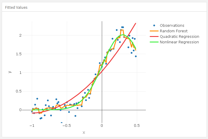
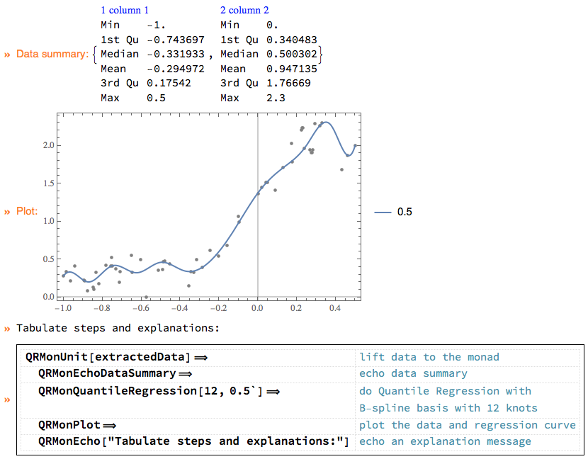
In this notebook/document we apply the monad QRMon [3] over data of the article [1]. In order to get the data we use extraction procedure described in [2].
TraceMonadUnit[QRMonUnit[extractedData]]⟹"lift data to the monad"⟹ QRMonEchoDataSummary⟹"echo data summary"⟹ QRMonQuantileRegression[12, 0.5]⟹"do Quantile Regression with\nB-spline basis with 12 knots"⟹ QRMonPlot⟹"plot the data and regression curve"⟹ QRMonEcho[Style["Tabulate QRMon steps and explanations:", Purple, Bold]]⟹"echo an explanation message"⟹ TraceMonadEchoGrid;