Autoencoder in TensorFlow 2: Beginner’s Guide

Imagine you have an image or an audio file which you would like to transfer to a friend. Sending the raw format data could be time-consuming and potentially inefficient, especially when the files’ size is big. What if we can convert these original bits into compressed formats at the source, making the transfer at a much faster speed? That’s right! An Autoencoder does just that for us, saves valuable space and makes sending files faster instead of having this bottleneck where transfer of data is slower as it is uncompressed. This post discusses Autoencoder in TensorFlow v2.4.

Before we get into the technical details of Autoencoder, let us look at some interesting applications it is used in:

• Remove noise from an image (denoising).

• Fill in the missing pieces in an image (Image Inpainting).

• Dimensionality reduction, clustering, and in recommender systems.
• A class of Autoencoder known as Variational Autoencoder can even learn to generate data! However, the vanilla Autoencoder fails to perform accurately due to shortcomings which we will discuss in this post.
• Autoencoders are used as a Feature Extractor for downstream tasks such as  classification, and detection.
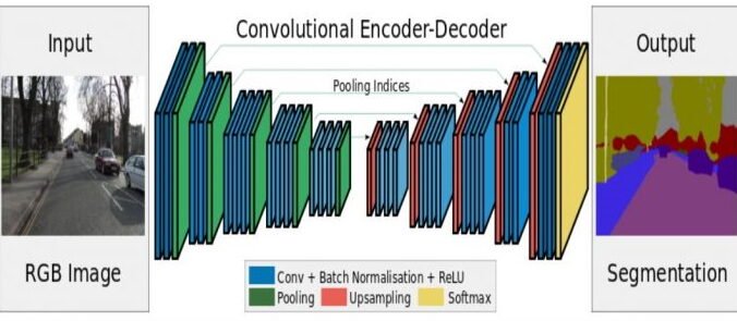
• Autoencoders are also widely leveraged in Semantic Segmentation. One such work SegNet was developed for multi-class pixel-wise segmentation on the urban road scene dataset. This work was published by members of the Computer Vision Group at the University of Cambridge. You can Try their demo here!

This article will discuss the following details of an Autoencoder in TensorFlow:

1. Introduction to Autoencoder in TensorFlow and how it works.
2. Discuss Autoencoder’s objective function.
3. Implement Autoencoder in TensorFlow using Fashion-MNIST Dataset.
4. Implement Autoencoder in TensorFlow using Google’s Cartoon Dataset.

Bonus

Not just the theory part and testing with datasets, let us dive deep. We will try to experimentally analyze the Autoencoder and develop a good understanding of its strength’s and weaknesses.

5. We will perform various experiments such as visualizing both the Autoencoder’s latent-space, generating images sampled from the latent-space: uniform and normal distribution.

6. With the results from step 3 and experiments in the above point, we will analyze and understand the Autoencoder’s strength and shortcomings.

7. Summary and Conclusion

What is an Autoencoder?

An Autoencoder is an unsupervised learning neural network. It is primarily used for learning data compression and inherently learns an identity function. First introduced in the 1980s, it was promoted in a paper by Hinton & Salakhutdinov in 2006. An Autoencoder network aims to learn a generalized latent representation ( encoding ) of a dataset. Autoencoder is helpful in various domains, such as for processing image, text, and audio.

100K+ Learners
3 Hours of Learning

Join Free OpenCV Bootcamp

15K+ Learners
3 Hours of Learning

Join Free TensorFlow Bootcamp

10K+ Learners
8 Hours of Learning

Join Free PyTorch Bootcamp

View all AI Free Courses

In an image domain, an Autoencoder is fed an image ( grayscale or color ) as input. The system reconstructs it using fewer bits. Autoencoders are similar in spirit to dimensionality reduction algorithms like the principal component analysis. They create a latent space where the necessary elements of the data are preserved while non-essential parts are filtered. An Autoencoder having one layer with no non-linearity can be considered a principal component analysis.

The Autoencoder network has two blocks:

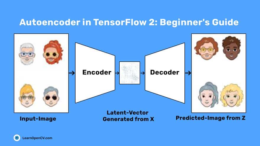
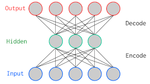
1. Encoder: This is the part of the network that compresses the input into a fewer number of bits known as latent-space, also sometimes called a bottleneck. This latent-space representation is called an “encoding” of the input.
2. Decoder: It is the part of the network that reconstructs the input image from the compressed representation.

The above picture shows a vanilla Autoencoder. It has a 2-layer Autoencoder and one hidden layer. Note that the input and output layers have the same number of neurons. The Autoencoder will take five actual values. The input is compressed into three real values at the bottleneck (middle layer). The decoder tries to reconstruct the five real values fed as an input to the network from the compressed values.

In practice, there are far more hidden layers between the input and the output.

Objective Function of Autoencoder in TensorFlow

The Autoencoder network is trained to obtain weights for the encoder and decoder that best minimizes the loss between the original input and the input reconstruction after it has passed through the encoder and decoder.

Consider in an Autoencoder the encoder function has parameters and the decoder function consists of parameters which are learned during the training. The low-dimensional code learned for input in the latent-space is and the reconstructed input is .

Both the encoder and decoder weights are learned in tandem to output a reconstructed image expected to be the same as the original input image, inherently learning an identity function . There are various metrics to quantify the difference between two vectors, but the one commonly used in Autoencoder is called Mean Squared Error ( MSE ).

The MSE loss is given as:

(1)  

In the above equation, is the number of images in your dataset or the mini-batch across which the loss is computed. MSE computes the pixel-wise difference between the original and the reconstructed output, raises the difference to the power of two, and takes an average over the full-batch or mini-batch of the data.

There are various kinds of Autoencoders like

• Vanilla Autoencoder
• Denoising Autoencoder
• Stacked or Sparse Autoencoder
• Contrastive Autoencoder
• Variational Autoencoder

Let us now move onto implementing a vanilla Autoencoder for reconstructing Fashion-MNIST and Cartoon images in TensorFlow, let us execute Autoencoder in TensorFlow.

Autoencoder in TensorFlow with Fashion-MNIST dataset

We will use the famous Fashion-MNIST dataset for implementing a vanilla Autoencoder for reconstruction.

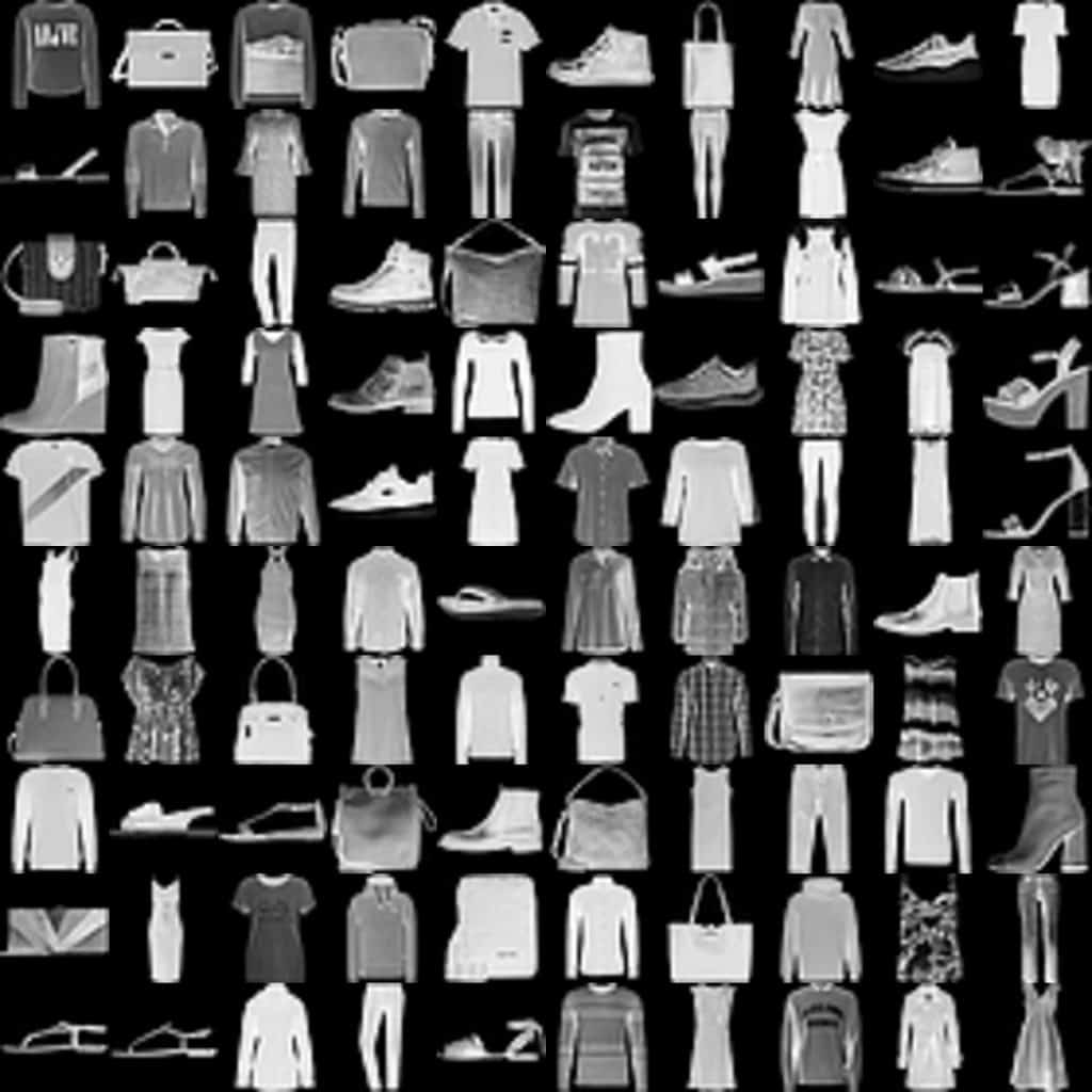
The Fashion-MNIST dataset consists of:

• Database of 60,000 fashion images shown on the right.
• Each image of size 28×28 ( grayscale ) is associated with a label from 10 categories such as t-shirt, trouser, and sneaker.

Note: All the implementations were carried out on an 11GB Pascal 1080Ti GPU.

Click here to download the source code to this post

Importing Modules

 # import the necessary packages import imageio import glob import os import time import cv2 import tensorflow as tf from tensorflow.keras import layers from IPython import display import matplotlib.pyplot as plt import numpy as np %matplotlib inline from tensorflow import keras 

We begin by importing necessary packages imageio, glob, tensorflow, tensorflow layers, time, and matplotlib for plotting on Lines 2-10.

Loading and Preprocessing Dataset

 (x_train, y_train), (x_test, y_test) = tf.keras.datasets.fashion_mnist.load_data() x_train = x_train.reshape(x_train.shape[0], 28, 28, 1).astype('float32') x_test = x_test.astype('float32') x_train = x_train / 255. x_test = x_test / 255. # Batch and shuffle the data train_dataset = tf.data.Dataset.from_tensor_slices(x_train).\ shuffle(60000).batch(128) 

Loading the dataset is relatively a simple task; use the tf_keras datasets module, which loads the data off-the-shelf. Since we do not require the labels to solve this problem, we will use the training images x_train. In Line 15, we reshape the images and cast them to float32 since the data is inherently in uint8 format.

Then, in Line 17-18, you normalize the data from [0, 255] to [0, 1]. Finally, we build the TensorFlow input pipeline. In essence, tf.data.Dataset.from_tensor_slices is fed the training data, shuffled, sliced into tensors. The processing allows us to access tensors of specified batch size during training. The buffer size ( 60000 ) parameter in shuffle affects the randomness of the shuffle.

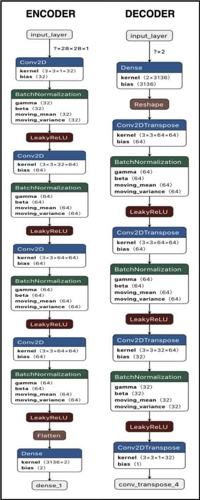
Architectural Diagram of Autoencoder in TensorFlow

Define the Encoder Network

 def encoder(input_encoder): inputs = keras.Input(shape=input_encoder, name='input_layer') # Block 1 x = layers.Conv2D(32, kernel_size=3, strides= 1, padding='same', name='conv_1')(inputs) x = layers.BatchNormalization(name='bn_1')(x) x = layers.LeakyReLU(name='lrelu_1')(x) # Block 2 x = layers.Conv2D(64, kernel_size=3, strides= 2, padding='same', name='conv_2')(x) x = layers.BatchNormalization(name='bn_2')(x) x = layers.LeakyReLU(name='lrelu_2')(x) # Block 3 x = layers.Conv2D(64, 3, 2, padding='same', name='conv_3')(x) x = layers.BatchNormalization(name='bn_3')(x) x = layers.LeakyReLU(name='lrelu_3')(x) # Block 4 x = layers.Conv2D(64, 3, 1, padding='same', name='conv_4')(x) x = layers.BatchNormalization(name='bn_4')(x) x = layers.LeakyReLU(name='lrelu_4')(x) # Final Block flatten = layers.Flatten()(x) bottleneck = layers.Dense(2, name='dense_1')(flatten) model = tf.keras.Model(inputs, bottleneck, name="Encoder") return model 

Here, we define the encoder network, which takes an input of size [None, 256, 256, 3]. There are five Conv blocks, each consisting of a Conv2D, BatchNorm and LeakyReLU activation function. In each block, the image is down sampled by a factor of two.

In the final block or the Flatten layer, we convert the [None, 8, 8, 64] to a vector of size 4096 and add a Dense layer of 200 neurons, also known as the Bottleneck ( Latent-Space ) layer. The bottleneck consists of 200 real values. We can also say that an image of size 256 x 256 x 3 is encoded or represented by 200 real values.

Define the Decoder Network

 def decoder(input_decoder): # Initial Block inputs = keras.Input(shape=input_decoder, name='input_layer') x = layers.Dense(3136, name='dense_1')(inputs) x = tf.reshape(x, [-1, 7, 7, 64], name='Reshape_Layer') # Block 1 x = layers.Conv2DTranspose(64, 3, strides= 1, padding='same',name='conv_transpose_1')(x) x = layers.BatchNormalization(name='bn_1')(x) x = layers.LeakyReLU(name='lrelu_1')(x) # Block 2 x = layers.Conv2DTranspose(64, 3, strides= 2, padding='same', name='conv_transpose_2')(x) x = layers.BatchNormalization(name='bn_2')(x) x = layers.LeakyReLU(name='lrelu_2')(x) # Block 3 x = layers.Conv2DTranspose(32, 3, 2, padding='same', name='conv_transpose_3')(x) x = layers.BatchNormalization(name='bn_3')(x) x = layers.LeakyReLU(name='lrelu_3')(x) # Block 4 outputs = layers.Conv2DTranspose(1, 3, 1,padding='same', activation='sigmoid', name='conv_transpose_4')(x) model = tf.keras.Model(inputs, outputs, name="Decoder") return model 

The decoder network takes an input of size [None, 200]. The initial block has a Dense layer having 4096 neurons. Recall that this was the size of the vector in the encoder function after flattening the output from the last conv block. There are a total of five Conv blocks. The Conv block [1, 4] consists of a Conv2DTranspose, BatchNorm and LeakyReLU activation function. The Conv block 5 has a Conv2DTranspose with sigmoid activation function, which flattens  the output to be in the range [0, 1]. In each block, the image is up sampled by a factor of two.

The decoder network’s output is a tensor of size [None, 28, 28, 1].

Optimizer and Loss Function

 optimizer = tf.keras.optimizers.Adam(lr = 0.0005) def ae_loss(y_true, y_pred): loss = K.mean(K.square(y_true - y_pred), axis = [1,2,3]) return loss 

We optimize the Autoencoder with Adam optimizer. The optimizer uses  an argument: a learning rate of . In Line 96, we define the autoencoder loss function, i.e., mean-squared error, which takes two arguments: the original image and reconstructed image.

Training the Autoencoder in TensorFlow

 # Notice the use of `tf.function` # This annotation causes the function to be "compiled". @tf.function def train_step(images): with tf.GradientTape() as encoder, tf.GradientTape() as decoder: latent = enc(images, training=True) generated_images = dec(latent, training=True) loss = ae_loss(images, generated_images) gradients_of_enc = encoder.gradient(loss, enc.trainable_variables) gradients_of_dec = decoder.gradient(loss, dec.trainable_variables) optimizer.apply_gradients(zip(gradients_of_enc, enc.trainable_variables)) optimizer.apply_gradients(zip(gradients_of_dec, dec.trainable_variables)) return loss 

In the above training loop, we train the encoder and decoder separately. We first pass the image to the encoder, and then the latent-space is fed to the decoder. The loss is computed over the images generated by the decoder.

Next, in Line 90-91, we compute the gradients and update the encoder & decoder parameters using the Adam optimizer. Finally, we return the loss.

 def train(dataset, epochs): for epoch in range(epochs): start = time.time() for image_batch in dataset: train_step(image_batch) print ('Time for epoch {} is {} sec'.format(epoch + 1, time.time()-start)) train(train_dataset, epoch) 

Finally, we train our Autoencoder model. The above train function takes the train_dataset and Epochs as the parameters and calls the train_step function at every new batch in total ( Total Training Images / Batch Size).

Reconstructing Test Images

Let us now test how well the model has learned to reconstruct the fashion images. We will use the test images, which are normalized in the range [0, 1]. Matplotlib will plot the images in a 5 x 5 grid.

With every reconstructed output, we will also plot their respective ground truth or label to judge the model’s performance.

 figsize = 15 latent = enc.predict(x_test[:25]) reconst = dec.predict(latent) fig = plt.figure(figsize=(figsize, 10)) for i in range(25): ax = fig.add_subplot(5, 5, i+1) ax.axis('off') ax.text(0.5, -0.15, str(label_dict[y_test[i]]), fontsize=10, ha='center', transform=ax.transAxes) ax.imshow(reconst[i, :,:,0]*255, cmap = 'gray')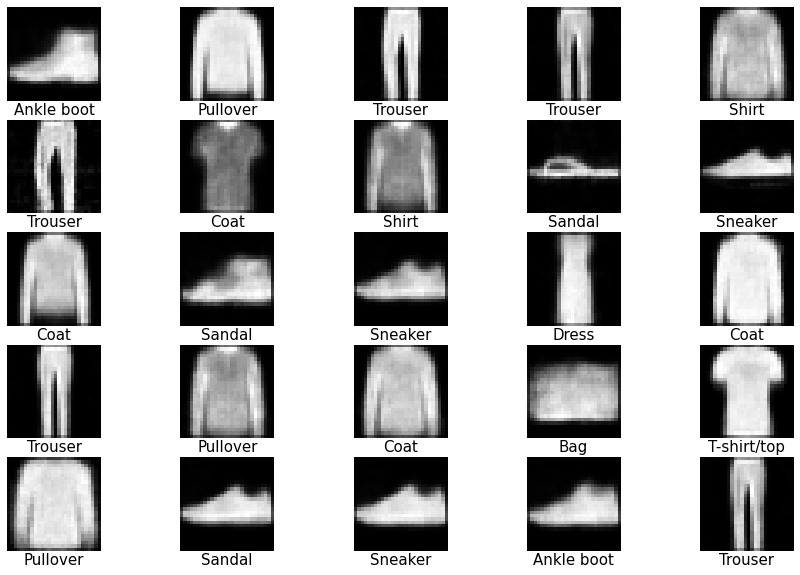 

From the above output, we can observe that the model did a great job of reconstructing the test images ( validating from the labels )

We will do a couple of more tests with our Fashion-MNIST Autoencoder in the later part of the tutorial. Feel free to jump directly to the test section.

Autoencoder with Cartoon Set Data

This section will only show the data loading, data preprocessing, encoder and decoder architecture since all other implementation parts are similar to the Fashion-MNIST implementation.

Dataset

Cartoon Set is a collection of random 2D cartoon avatar RGB images. The collection has:

• 10 artwork categories,
• 4 color categories, and 
• 4 proportion categories,

The dataset comes with ~10¹³ possible combinations. The images are of fixed-size, i.e., 512 x 512 x 3. It has two sets: 10k and 100k randomly chosen cartoons and labeled attributes. We would be using the 100k image set for training the Autoencoder.

Loading and Preprocessing the Data

 train_ds = tf.keras.preprocessing.image_dataset_from_directory( 'cartoonset100k', image_size=(256, 256), batch_size=batch_size, label_mode=None) normalization_layer = layers.experimental.preprocessing.Rescaling(scale= 1./255) normalized_ds = train_ds.map(lambda x: normalization_layer(x)) 

Loading the dataset is a fairly simple task; use the tf_keras preprocessing dataset module, which has a function image_dataset_from_directory. It loads the data from the specified directory, which in our case is cartoonset100k. We pass the required image_size [256, 256, 3] and batch_size ( 128 ), at which we will train our model. Since this is an unsupervised problem, we do not use the labels and label_mode flag as None.

Finally, in Line 9, we use the Lambda function to normalize all the input images from [0, 255] to [0, 1] and get normalized_ds which we will use for training our model. In the Lambda function, we pass the preprocessing layer defined at Line 7.

Autoencoder in TensorFlow – Architecture

The encoder’s input is [None, 256, 256, 3], and the bottleneck or the latent-space has 200 neurons. The decoder feeds on an input of [None, 200]. This input is upsampled to produce an image similar to the input

Define the Encoder Network

 def encoder(input_encoder): inputs = keras.Input(shape=input_encoder, name='input_layer') # Block 1 x = layers.Conv2D(32, kernel_size=3, strides= 2, padding='same', name='conv_1')(inputs) x = layers.BatchNormalization(name='bn_1')(x) x = layers.LeakyReLU(name='lrelu_1')(x) # Block 2 x = layers.Conv2D(64, kernel_size=3, strides= 2, padding='same', name='conv_2')(x) x = layers.BatchNormalization(name='bn_2')(x) x = layers.LeakyReLU(name='lrelu_2')(x) # Block 3 x = layers.Conv2D(64, 3, 2, padding='same', name='conv_3')(x) x = layers.BatchNormalization(name='bn_3')(x) x = layers.LeakyReLU(name='lrelu_3')(x) # Block 4 x = layers.Conv2D(64, 3, 2, padding='same', name='conv_4')(x) x = layers.BatchNormalization(name='bn_4')(x) x = layers.LeakyReLU(name='lrelu_4')(x) # Block 5 x = layers.Conv2D(64, 3, 2, padding='same', name='conv_5')(x) x = layers.BatchNormalization(name='bn_5')(x) x = layers.LeakyReLU(name='lrelu_5')(x) # Final Block flatten = layers.Flatten()(x) bottleneck = layers.Dense(200, name='dense_1')(flatten) model = tf.keras.Model(inputs, bottleneck, name="Encoder") return model 

Here, we define the encoder network, which takes an input of size [None, 256, 256, 3]. There are five Conv blocks, each consisting of a Conv2D, BatchNorm and LeakyReLU activation function. In each block, the image is down sampled by a factor of two.

In the final block or the Flatten layer, we convert the [None, 8, 8, 64] to a vector of size 4096 and add a Dense layer of 200 neurons, also known as the Bottleneck ( Latent-Space ) layer. The bottleneck consists of 200 real values. We can also say that an image of size 256 x 256 x 3 is encoded or represented by 200 real values.

Define the Decoder Network

 def decoder(input_decoder): # Initial Block inputs = keras.Input(shape=input_decoder, name='input_layer') x = layers.Dense(4096, name='dense_1')(inputs) x = tf.reshape(x, [-1, 8, 8, 64], name='Reshape_Layer') # Block 1 x = layers.Conv2DTranspose(64, 3, strides= 2, padding='same',name='conv_transpose_1')(x) x = layers.BatchNormalization(name='bn_1')(x) x = layers.LeakyReLU(name='lrelu_1')(x) # Block 2 x = layers.Conv2DTranspose(64, 3, strides= 2, padding='same', name='conv_transpose_2')(x) x = layers.BatchNormalization(name='bn_2')(x) x = layers.LeakyReLU(name='lrelu_2')(x) # Block 3 x = layers.Conv2DTranspose(64, 3, 2, padding='same', name='conv_transpose_3')(x) x = layers.BatchNormalization(name='bn_3')(x) x = layers.LeakyReLU(name='lrelu_3')(x) # Block 4 x = layers.Conv2DTranspose(32, 3, 2, padding='same', name='conv_transpose_4')(x) x = layers.BatchNormalization(name='bn_4')(x) x = layers.LeakyReLU(name='lrelu_4')(x) # Block 5 outputs = layers.Conv2DTranspose(3, 3, 2,padding='same', activation='sigmoid', name='conv_transpose_5')(x) model = tf.keras.Model(inputs, outputs, name="Decoder") return model 

The decoder network takes an input of size [None, 200]. The initial block has a Dense layer having 4096 neurons. Recall that this was the size of the vector in the encoder function after flattening the output from the last conv block. There are a total of five Conv blocks. The Conv block [1, 4] consists of a Conv2DTranspose, BatchNorm and LeakyReLU activation function. The Conv block 5 has a Conv2DTranspose with sigmoid activation function, which flattens  the output to be in the range [0, 1]. In each block, the image is up sampled by a factor of two.

The decoder network’s output  is a tensor of size [None, 256, 256, 3].

Reconstructing the Cartoon Images

Its time to test our Autoencoder model by reconstructing the cartoon images.

 reconstruction = None lat_space = None for i in normalized_ds: latent= enc.predict(i) out = dec.predict(latent) if reconstruction is None: reconstruction = out lat_space = latent else: reconstruction = np.concatenate((reconstruction, out)) lat_space = np.concatenate((lat_space, latent)) if reconstruction.shape[0] > 5000: break 

We define two variables, reconstruction and lat_space,  which will store the reconstructed images and the latent-space encoding, respectively. At Line 77, we iterate over the dataset normalized_ds only up to a little over 5000 images. Since we defined encoder and decoder separately, we pass the images first to the enc model and then its output is fed to the dec model.

We store the encodings as well since we will be visualizing and analyzing the latent space.

 figsize = 15 fig = plt.figure(figsize=(figsize, 10)) for i in range(25): ax = fig.add_subplot(5, 5, i+1) ax.axis('off') pred = reconstruction[i, :, :, :] * 255 pred = np.array(pred) pred = pred.astype(np.uint8) ax.imshow(pred)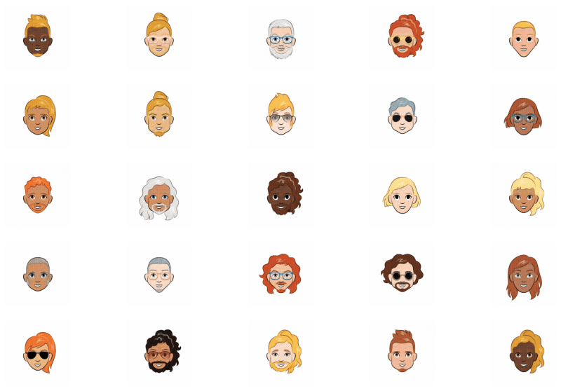 

It looks like the Autoencoder did a great job at reconstructing the images. Even the finer details are sharp and perceptually good, given that the Cartoon Set compared to the Fashion-MNIST is complex.

100K+ Learners
3 Hours of Learning

Join Free OpenCV Bootcamp

15K+ Learners
3 Hours of Learning

Join Free TensorFlow Bootcamp

10K+ Learners
8 Hours of Learning

Join Free PyTorch Bootcamp

View all AI Free Courses

Visualizing the Latent Space of Autoencoder in TensorFlow

This section will visualize Autoencoder’s latent space trained on both Fashion-MNIST and Cartoon Set Data. We will try to develop some intuition about the gaps that prevent Autoencoders from being generative in nature.

Latent Space Projection of Autoencoder in TensorFlow, Trained on Fashion-MNIST

 imgs_visualize = 5000 figsize = 10 index = np.random.choice(range(len(x_test)), imgs_visualize) images = x_test[index] embeddings = enc.predict(images) plt.figure(figsize=(figsize, figsize)) plt.scatter(embeddings[:, 0] , embeddings[:, 1], alpha=0.5, s=2) plt.xlabel("Dimension-1", size=20) plt.ylabel("Dimension-2", size=20) plt.xticks(size=20) plt.yticks(size=20) plt.title("Projection of 2D Latent-Space (Fashion-MNIST)", size=20) plt.show()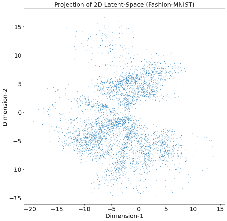 

We randomly chose 5K images from the 10K test set of Fashion-MNIST and fed them  to the encoder.  It outputs an embeddings vector of shape [5000, 2]. We plot these 5K embeddings on the x and y axes as shown in the above scatter plot.

The above scatter plot does not appear to be symmetrical around the point [0, 0] and is not bounded. Dimension-1 has values in the range [-20, 15] and dimension-2 has values in the range [-15, 15]. Many data points lie in the negative region of the latent-space, while only a few data points lie in the positive region.

We can also see some outliers that are far from the other data points and lie on each dimension’s extremes.

Our goal is to choose a random point in the latent space or sample a vector with normal distribution, feed this to the trained decoder, and expect it to produce an image that looks similar to the original Fashion Image. Autoencoder fails to meet our goal since we do not enforce any prior on the latent-space like it should be bounded, continuous, and follow any specific distribution.

We observe that our latent-space seems irregular and not continuous; there are significant gaps between the data points’ encodings. It is almost impossible to know which random point to pick from the latent space and decode it to generate a realistic fashion image since there are gaps in the latent space clusters. Hence, if we happen to pick a point from the gap and pass it to the decoder, it might give an arbitrary output ( or noise ) that doesn’t resemble any of the classes.

Latent Space Projection with t-SNE of Autoencoder in TensorFlow Trained on Cartoon Set

Now we will plot the latent-space of Autoencoder trained with Cartoon Set data. Since this Autoencoder’s bottleneck or latent-space is 200D we can not visualize it directly in a 2D graph. Hence, we first apply a dimensionality-reduction technique known as t-Stochastic Network Embeddings (t-SNE), which projects the 200D latent-space into a 2D space by preserving the relevant information.

 tsne = TSNE(n_components=2, init='pca', random_state=0) X_tsne = tsne.fit_transform(embeddings) plt.figure(figsize=(figsize, figsize)) plt.scatter(X_tsne[:, 0] , X_tsne[:, 1], alpha=0.5, s=2) plt.show()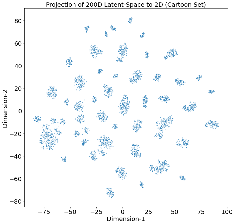 

We choose 5K images and feed them to the decoder trained on Cartoon Set data. From the above plot, we can gather similar observations as noted in our previous experiment. The latent-space has major gaps. It is discontinuous and is unbounded. Dimension-1 has values in the range [-75, 100] and dimension-2 has values in the range [-80, 80].

We can expect some error due to the post-processing, i.e., dimensionality-reduction. Still, given the pattern we see in the above visualization ( a lot of gaps ), the post-processing error could be ignored. Moreover, we would be performing similar sets of experiments in our next tutorial on Variational Autoencoder, and we will see if we get a continuous latent-space after applying t-SNE or not.

Reconstructing Images Randomly from Latent Spaces

Reconstructing Fashion Images with Latent-Vector Sampled Uniformly

We will take the lower bound and upper bound from the fashion-mnist latent-space ( two dimensions ) and sample two NumPy arrays, each of size [10, 1] with a uniform distribution. We will concatenate these arrays x and y respectively and feed them to the decoder.

Finally, we will plot these images.

 min_x = min(embeddings[:, 0]) max_x = max(embeddings[:, 0]) min_y = min(embeddings[:, 1]) max_y = max(embeddings[:, 1]) x = np.random.uniform(low=min_x,high=max_x, size = (10,1)) y = np.random.uniform(low=min_y,high=max_y, size = (10,1)) bottleneck = np.concatenate((x, y), axis=1) reconst = dec.predict(bottleneck) fig = plt.figure(figsize=(15, 10)) for i in range(10): ax = fig.add_subplot(5, 5, i+1) ax.axis('off') ax.text(0.5, -0.15, str(np.round(bottleneck[i],1)), fontsize=10, ha='center', transform=ax.transAxes) ax.imshow(reconst[i, :,:,0]*255, cmap = 'gray') 

The above outputs are not well reconstructed. They are blurry, pixelated, and not well-formed. For example, the second row and third column image seem like a Trouser, but the reconstructed image is not even close to being a Trouser.

We might argue that some of these images latent-space points might lie on the boundary, which could be the reason for them being poorly reconstructed. However, even if the latent-space points lie in the center, we cannot expect the reconstruction to be good. The latent-space of the Autoencoder is not continuous.

Reconstructing Cartoon Images with Latent-Vector Sampled Uniformly

To sample a point uniformly from a latent-space of 200D, we cannot simply pass the lower bound and upper bound to np.random.uniform(). We will need to do this for all 200D. Instead, we take the minimum and maximum of the 200D across all 5K images, sample a uniform matrix of size [10, 200] whose values lie between [0, 1]. We then scale these values by taking the difference between the minimum and maximum of the latent-space. We then pass the scaled output to the decoder and generate the images.

 figsize = 15 min_x = lat_space.min(axis=0) max_x = lat_space.max(axis=0) input = np.random.uniform(size = (10,200)) bottleneck = x * (max_x - (np.abs(min_x))) print(x.shape) reconstruct = dec.predict(bottleneck) fig = plt.figure(figsize=(figsize, 10)) for i in range(10): ax = fig.add_subplot(5, 5, i+1) ax.axis('off') pred = reconstruct[i, :, :, :] * 255 pred = np.array(pred) pred = pred.astype(np.uint8) ax.imshow(pred) 

We can see that images reconstructed are poor, blurry, and perceptually not good. One could compare them with images reconstructed by the Autoencoder during the training, and the difference would be noticeable.

Let us do one last experiment!

Reconstructing Cartoon Images from a Latent-Vector Sampled with Normal Distribution

Here we will sample an array of size [10, 200] from a normal distribution and feed it to the decoder.

Let us find out the result.

 x = np.random.normal(size = (10,200)) reconstruct = dec.predict(x) fig = plt.figure(figsize=(15, 10)) fig.subplots_adjust(hspace=0.2, wspace=0.2) for i in range(10): ax = fig.add_subplot(5, 5, i+1) ax.axis('off') pred = reconstruct[i, :, :, :] * 255 pred = np.array(pred) pred = pred.astype(np.uint8) ax.imshow(pred) 

As expected, the reconstructions are even worse, or rather the Autoencoder failed to reconstruct anything meaningful. The reason is that we are not enforcing a prior on the Autoencoder’s latent-space to be normally distributed. Also, the parameters ( weights ) learned by the decoder do not expect latent-space values to have a mean of zero and variance of one.

Conclusion

Fantastic, an avid reader and a staunch learner that you are! I want to thank you and congratulate you on making it this far. We know it was a lot to take in. Let us quickly summarize our learning’s.

1. We started off by introducing you to the applications of Autoencoder.
2. We discussed the core idea behind Autoencoder and how it functions.
3. Then we discussed the objective function of the Autoencoder, i.e., mean-squared error.
4. Implemented an Autoencoder in TensorFlow and tested it using two datasets: Fashion-MNIST and the Cartoon Set.
5. We did various experiments like visualizing both the Autoencoders’ latent-space, generating images sampled uniformly from the latent-space.
6. We also tried generating cartoon images with a latent-vector sampled from a normal distribution and learned that Autoencoder fails to generate images when sampled from a normal distribution. We also learned that vanilla Autoencoder is not very generative in nature.
7. By doing these experiments, we learned a lot about Autoencoder’s inner working and its shortcomings.

Did you get any ideas and strategies after completing this post? Do you have any exciting ideas to improve the working or overcome the shortcomings of Autoencoder? Any plan to try (implement) them? Let us know in the comments.