Visualize predictions with tables
6 minute read
This covers how to track, visualize, and compare model predictions over the course of training, using PyTorch on MNIST data.
You will learn how to:
- Log metrics, images, text, etc. to a
wandb.Table()during model training or evaluation - View, sort, filter, group, join, interactively query, and explore these tables
- Compare model predictions or results: dynamically across specific images, hyperparameters/model versions, or time steps.
Examples
Compare predicted scores for specific images
Live example: compare predictions after 1 vs 5 epochs of training →
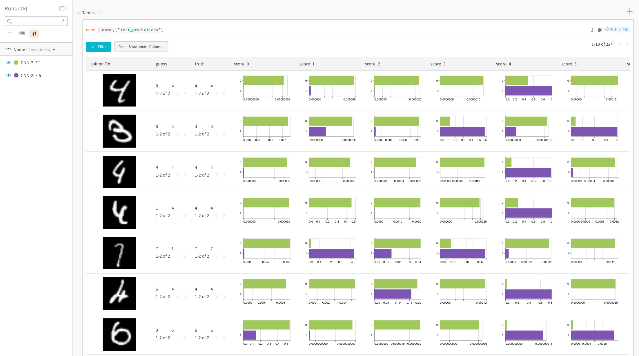
The histograms compare per-class scores between the two models. The top green bar in each histogram represents model “CNN-2, 1 epoch” (id 0), which only trained for 1 epoch. The bottom purple bar represents model “CNN-2, 5 epochs” (id 1), which trained for 5 epochs. The images are filtered to cases where the models disagree. For example, in the first row, the “4” gets high scores across all the possible digits after 1 epoch, but after 5 epochs it scores highest on the correct label and very low on the rest.
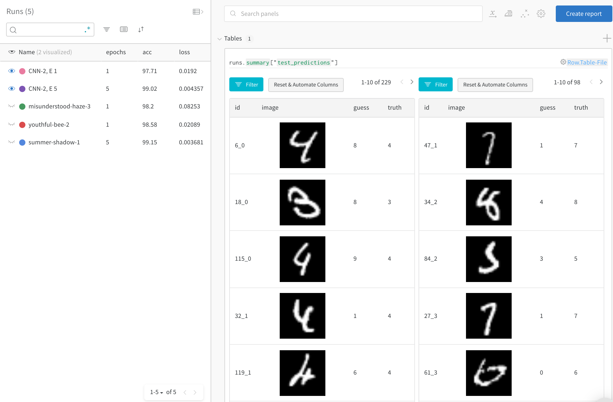
Focus on top errors over time
See incorrect predictions (filter to rows where “guess” != “truth”) on the full test data. Note that there are 229 wrong guesses after 1 training epoch, but only 98 after 5 epochs.
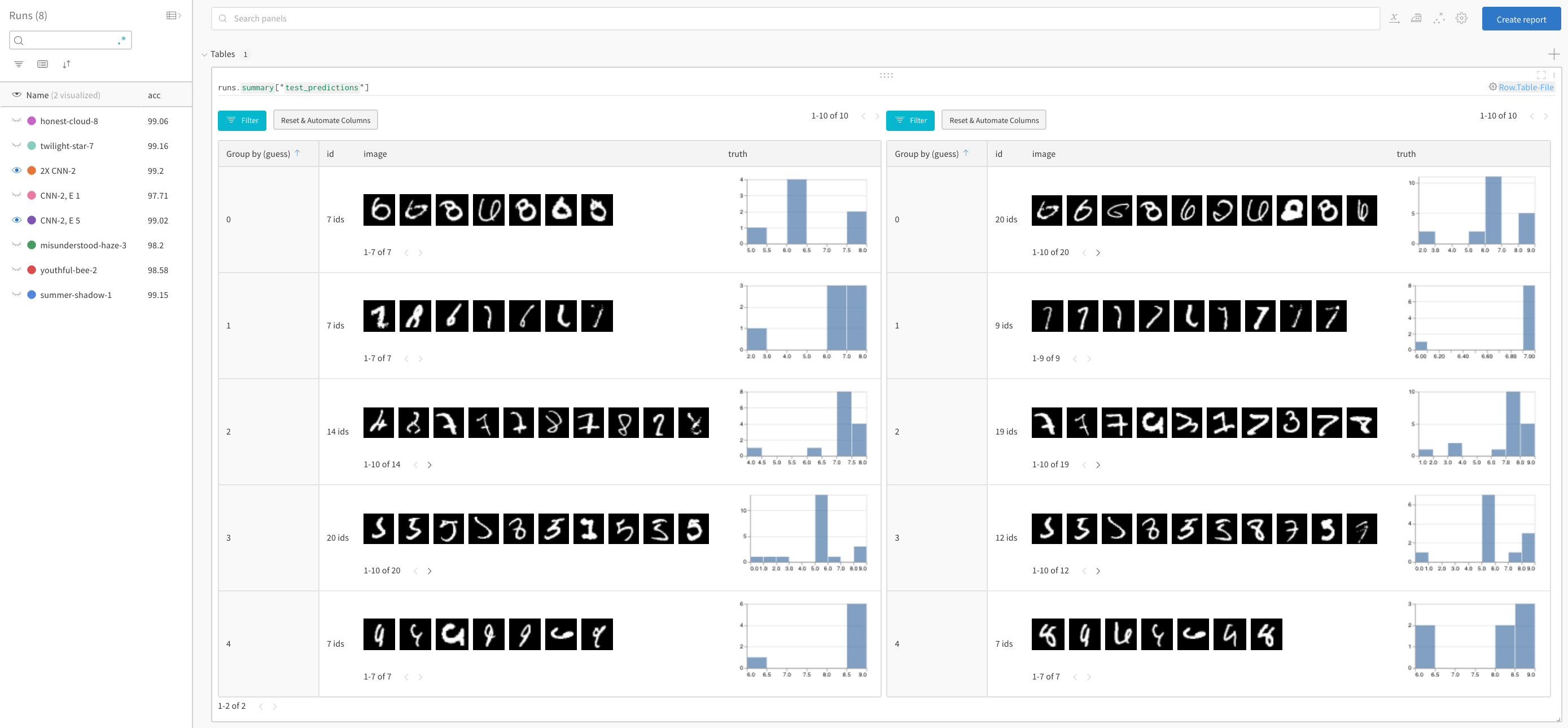
Compare model performance and find patterns
See full detail in a live example →
Filter out correct answers, then group by the guess to see examples of misclassified images and the underlying distribution of true labels—for two models side-by-side. A model variant with 2X the layer sizes and learning rate is on the left, and the baseline is on the right. Note that the baseline makes slightly more mistakes for each guessed class.
Sign up or login
Sign up or login to W&B to see and interact with your experiments in the browser.
In this example we’re using Google Colab as a convenient hosted environment, but you can run your own training scripts from anywhere and visualize metrics with W&B’s experiment tracking tool.
!pip install wandb -qqq log to your account
import wandb wandb.login() WANDB_PROJECT = "mnist-viz" 0. Setup
Install dependencies, download MNIST, and create train and test datasets using PyTorch.
import torch import torch.nn as nn import torchvision import torchvision.transforms as T import torch.nn.functional as F device = "cuda:0" if torch.cuda.is_available() else "cpu" # create train and test dataloaders def get_dataloader(is_train, batch_size, slice=5): "Get a training dataloader" ds = torchvision.datasets.MNIST(root=".", train=is_train, transform=T.ToTensor(), download=True) loader = torch.utils.data.DataLoader(dataset=ds, batch_size=batch_size, shuffle=True if is_train else False, pin_memory=True, num_workers=2) return loader 1. Define the model and training schedule
- Set the number of epochs to run, where each epoch consists of a training step and a validation (test) step. Optionally configure the amount of data to log per test step. Here the number of batches and number of images per batch to visualize are set low to simplify the demo.
- Define a simple convolutional neural net (following pytorch-tutorial code).
- Load in train and test sets using PyTorch
# Number of epochs to run # Each epoch includes a training step and a test step, so this sets # the number of tables of test predictions to log EPOCHS = 1 # Number of batches to log from the test data for each test step # (default set low to simplify demo) NUM_BATCHES_TO_LOG = 10 #79 # Number of images to log per test batch # (default set low to simplify demo) NUM_IMAGES_PER_BATCH = 32 #128 # training configuration and hyperparameters NUM_CLASSES = 10 BATCH_SIZE = 32 LEARNING_RATE = 0.001 L1_SIZE = 32 L2_SIZE = 64 # changing this may require changing the shape of adjacent layers CONV_KERNEL_SIZE = 5 # define a two-layer convolutional neural network class ConvNet(nn.Module): def __init__(self, num_classes=10): super(ConvNet, self).__init__() self.layer1 = nn.Sequential( nn.Conv2d(1, L1_SIZE, CONV_KERNEL_SIZE, stride=1, padding=2), nn.BatchNorm2d(L1_SIZE), nn.ReLU(), nn.MaxPool2d(kernel_size=2, stride=2)) self.layer2 = nn.Sequential( nn.Conv2d(L1_SIZE, L2_SIZE, CONV_KERNEL_SIZE, stride=1, padding=2), nn.BatchNorm2d(L2_SIZE), nn.ReLU(), nn.MaxPool2d(kernel_size=2, stride=2)) self.fc = nn.Linear(7*7*L2_SIZE, NUM_CLASSES) self.softmax = nn.Softmax(NUM_CLASSES) def forward(self, x): # uncomment to see the shape of a given layer: #print("x: ", x.size()) out = self.layer1(x) out = self.layer2(out) out = out.reshape(out.size(0), -1) out = self.fc(out) return out train_loader = get_dataloader(is_train=True, batch_size=BATCH_SIZE) test_loader = get_dataloader(is_train=False, batch_size=2*BATCH_SIZE) device = torch.device("cuda:0" if torch.cuda.is_available() else "cpu") 2. Run training and log test predictions
For every epoch, run a training step and a test step. For each test step, create a wandb.Table() in which to store test predictions. These can be visualized, dynamically queried, and compared side by side in your browser.
# convenience funtion to log predictions for a batch of test images def log_test_predictions(images, labels, outputs, predicted, test_table, log_counter): # obtain confidence scores for all classes scores = F.softmax(outputs.data, dim=1) log_scores = scores.cpu().numpy() log_images = images.cpu().numpy() log_labels = labels.cpu().numpy() log_preds = predicted.cpu().numpy() # adding ids based on the order of the images _id = 0 for i, l, p, s in zip(log_images, log_labels, log_preds, log_scores): # add required info to data table: # id, image pixels, model's guess, true label, scores for all classes img_id = str(_id) + "_" + str(log_counter) test_table.add_data(img_id, wandb.Image(i), p, l, *s) _id += 1 if _id == NUM_IMAGES_PER_BATCH: break # W&B: Initialize a new run to track this model's training with wandb.init(project="table-quickstart") as run: # W&B: Log hyperparameters using config cfg = run.config cfg.update({"epochs" : EPOCHS, "batch_size": BATCH_SIZE, "lr" : LEARNING_RATE, "l1_size" : L1_SIZE, "l2_size": L2_SIZE, "conv_kernel" : CONV_KERNEL_SIZE, "img_count" : min(10000, NUM_IMAGES_PER_BATCH*NUM_BATCHES_TO_LOG)}) # define model, loss, and optimizer model = ConvNet(NUM_CLASSES).to(device) criterion = nn.CrossEntropyLoss() optimizer = torch.optim.Adam(model.parameters(), lr=LEARNING_RATE) # train the model total_step = len(train_loader) for epoch in range(EPOCHS): # training step for i, (images, labels) in enumerate(train_loader): images = images.to(device) labels = labels.to(device) # forward pass outputs = model(images) loss = criterion(outputs, labels) # backward and optimize optimizer.zero_grad() loss.backward() optimizer.step() # W&B: Log loss over training steps, visualized in the UI live run.log({"loss" : loss}) if (i+1) % 100 == 0: print ('Epoch [{}/{}], Step [{}/{}], Loss: {:.4f}' .format(epoch+1, EPOCHS, i+1, total_step, loss.item())) # W&B: Create a Table to store predictions for each test step columns=["id", "image", "guess", "truth"] for digit in range(10): columns.append("score_" + str(digit)) test_table = wandb.Table(columns=columns) # test the model model.eval() log_counter = 0 with torch.no_grad(): correct = 0 total = 0 for images, labels in test_loader: images = images.to(device) labels = labels.to(device) outputs = model(images) _, predicted = torch.max(outputs.data, 1) if log_counter < NUM_BATCHES_TO_LOG: log_test_predictions(images, labels, outputs, predicted, test_table, log_counter) log_counter += 1 total += labels.size(0) correct += (predicted == labels).sum().item() acc = 100 * correct / total # W&B: Log accuracy across training epochs, to visualize in the UI run.log({"epoch" : epoch, "acc" : acc}) print('Test Accuracy of the model on the 10000 test images: {} %'.format(acc)) # W&B: Log predictions table to wandb run.log({"test_predictions" : test_table}) What’s next?
The next tutorial, you will learn how to optimize hyperparameters using W&B Sweeps.
Feedback
Was this page helpful?
Glad to hear it! If you have more to say, please let us know.
Sorry to hear that. Please tell us how we can improve.