Pandas Crosstab Explained
Posted by Chris Moffitt in articles
Introduction
Pandas offers several options for grouping and summarizing data but this variety of options can be a blessing and a curse. These approaches are all powerful data analysis tools but it can be confusing to know whether to use a groupby , pivot_table or crosstab to build a summary table. Since I have previously covered pivot_tables, this article will discuss the pandas crosstab function, explain its usage and illustrate how it can be used to quickly summarize data. My goal is to have this article be a resource that you can bookmark and refer to when you need to remind yourself what you can do with the crosstab function.
Overview
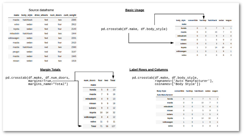
The pandas crosstab function builds a cross-tabulation table that can show the frequency with which certain groups of data appear. For a quick example, this table shows the number of two or four door cars manufactured by various car makers:
| num_doors | four | two | Total |
|---|---|---|---|
| make | |||
| honda | 5 | 8 | 13 |
| mazda | 7 | 9 | 16 |
| mitsubishi | 4 | 9 | 13 |
| nissan | 9 | 9 | 18 |
| subaru | 9 | 3 | 12 |
| toyota | 18 | 14 | 32 |
| volkswagen | 8 | 4 | 12 |
| volvo | 11 | 0 | 11 |
| Total | 71 | 56 | 127 |
In the table above, you can see that the data set contains 32 Toyota cars of which 18 are four door and 14 are two door. This is a relatively simple table to interpret and illustrates why this approach can be a powerful way to summarize large data sets.
Pandas makes this process easy and allows us to customize the tables in several different manners. In the rest of the article, I will walk through how to create and customize these tables.
Start the Process
Let’s get started by importing all the modules we need. If you want to follow along on your own, I have placed the notebook on github:
import pandas as pd import seaborn as sns Now we’ll read in the automobile data set from the UCI Machine Learning Repository and make some label changes for clarity:
# Define the headers since the data does not have any headers = ["symboling", "normalized_losses", "make", "fuel_type", "aspiration", "num_doors", "body_style", "drive_wheels", "engine_location", "wheel_base", "length", "width", "height", "curb_weight", "engine_type", "num_cylinders", "engine_size", "fuel_system", "bore", "stroke", "compression_ratio", "horsepower", "peak_rpm", "city_mpg", "highway_mpg", "price"] # Read in the CSV file and convert "?" to NaN df_raw = pd.read_csv("http://mlr.cs.umass.edu/ml/machine-learning-databases/autos/imports-85.data", header=None, names=headers, na_values="?" ) # Define a list of models that we want to review models = ["toyota","nissan","mazda", "honda", "mitsubishi", "subaru", "volkswagen", "volvo"] # Create a copy of the data with only the top 8 manufacturers df = df_raw[df_raw.make.isin(models)].copy() For this example, I wanted to shorten the table so I only included the 8 models listed above. This is done solely to make the article more compact and hopefully more understandable.
For the first example, let’s use pd.crosstab to look at how many different body styles these car makers made in 1985 (the year this dataset contains).
pd.crosstab(df.make, df.body_style) | body_style | convertible | hardtop | hatchback | sedan | wagon |
|---|---|---|---|---|---|
| make | |||||
| honda | 0 | 0 | 7 | 5 | 1 |
| mazda | 0 | 0 | 10 | 7 | 0 |
| mitsubishi | 0 | 0 | 9 | 4 | 0 |
| nissan | 0 | 1 | 5 | 9 | 3 |
| subaru | 0 | 0 | 3 | 5 | 4 |
| toyota | 1 | 3 | 14 | 10 | 4 |
| volkswagen | 1 | 0 | 1 | 9 | 1 |
| volvo | 0 | 0 | 0 | 8 | 3 |
The crosstab function can operate on numpy arrays, series or columns in a dataframe. For this example, I pass in df.make for the crosstab index and df.body_style for the crosstab’s columns. Pandas does that work behind the scenes to count how many occurrences there are of each combination. For example, in this data set Volvo makes 8 sedans and 3 wagons.
Before we go much further with this example, more experienced readers may wonder why we use the crosstab instead of a another pandas option. I will address that briefly by showing two alternative approaches.
First, we could use a groupby followed by an unstack to get the same results:
df.groupby(['make', 'body_style'])['body_style'].count().unstack().fillna(0) The output for this example looks very similar to the crosstab but it took a couple of extra steps to get it formatted correctly.
It is also possible to do something similar using a pivot_table :
df.pivot_table(index='make', columns='body_style', aggfunc={'body_style':len}, fill_value=0) Make sure to review my previous article on pivot_tables if you would like to understand how this works.
The question still remains, why even use a crosstab function? The short answer is that it provides a couple of handy functions to more easily format and summarize the data.
The longer answer is that sometimes it can be tough to remember all the steps to make this happen on your own. The simple crosstab API is the quickest route to the solution and provides some useful shortcuts for certain types of analysis.
In my experience, it is important to know about the options and use the one that flows most naturally from the analysis. I have had experiences where I struggled trying to make a pivot_table solution and then quickly got what I wanted by using a crosstab. The great thing about pandas is that once the data is in a dataframe all these manipulations are 1 line of code so you are free to experiment.
Diving Deeper into the Crosstab
Now that we have walked through the basic crosstab process, I will explain some of the other useful changes you can make to the output by altering the parameters.
One common need in a crosstab is to include subtotals. We can add them using the margins keyword:
pd.crosstab(df.make, df.num_doors, margins=True, margins_name="Total") | num_doors | four | two | Total |
|---|---|---|---|
| make | |||
| honda | 5 | 8 | 13 |
| mazda | 7 | 9 | 16 |
| mitsubishi | 4 | 9 | 13 |
| nissan | 9 | 9 | 18 |
| subaru | 9 | 3 | 12 |
| toyota | 18 | 14 | 32 |
| volkswagen | 8 | 4 | 12 |
| volvo | 11 | 0 | 11 |
| Total | 71 | 56 | 127 |
The margins keyword instructed pandas to add a total for each row as well as a total at the bottom. I also passed a value to margins_name in the function call because I wanted to label the results “Total” instead of the default “All”.
All of these examples have simply counted the individual occurrences of the data combinations. crosstab allows us to do even more summarization by including values to aggregate. To illustrate this, we can calculate the average curb weight of cars by body style and manufacturer:
pd.crosstab(df.make, df.body_style, values=df.curb_weight, aggfunc='mean').round(0) | body_style | convertible | hardtop | hatchback | sedan | wagon |
|---|---|---|---|---|---|
| make | |||||
| honda | NaN | NaN | 1970.0 | 2289.0 | 2024.0 |
| mazda | NaN | NaN | 2254.0 | 2361.0 | NaN |
| mitsubishi | NaN | NaN | 2377.0 | 2394.0 | NaN |
| nissan | NaN | 2008.0 | 2740.0 | 2238.0 | 2452.0 |
| subaru | NaN | NaN | 2137.0 | 2314.0 | 2454.0 |
| toyota | 2975.0 | 2585.0 | 2370.0 | 2338.0 | 2708.0 |
| volkswagen | 2254.0 | NaN | 2221.0 | 2342.0 | 2563.0 |
| volvo | NaN | NaN | NaN | 3023.0 | 3078.0 |
By using aggfunc='mean' and values=df.curb_weight we are telling pandas to apply the mean function to the curb weight of all the combinations of the data. Under the hood, pandas is grouping all the values together by make and body_style, then calculating the average. In those areas where there is no car with those values, it displays NaN . In this example, I am also rounding the results.
We have seen how to count values and determine averages of values. However, there is another common case of data sumarization where we want to understand the percentage of time each combination occurs. This can be accomplished using the normalize parameter:
pd.crosstab(df.make, df.body_style, normalize=True) | body_style | convertible | hardtop | hatchback | sedan | wagon |
|---|---|---|---|---|---|
| make | |||||
| honda | 0.000000 | 0.000000 | 0.054688 | 0.039062 | 0.007812 |
| mazda | 0.000000 | 0.000000 | 0.078125 | 0.054688 | 0.000000 |
| mitsubishi | 0.000000 | 0.000000 | 0.070312 | 0.031250 | 0.000000 |
| nissan | 0.000000 | 0.007812 | 0.039062 | 0.070312 | 0.023438 |
| subaru | 0.000000 | 0.000000 | 0.023438 | 0.039062 | 0.031250 |
| toyota | 0.007812 | 0.023438 | 0.109375 | 0.078125 | 0.031250 |
| volkswagen | 0.007812 | 0.000000 | 0.007812 | 0.070312 | 0.007812 |
| volvo | 0.000000 | 0.000000 | 0.000000 | 0.062500 | 0.023438 |
This table shows us that 2.3% of the total population are Toyota hardtops and 6.25% are Volvo sedans.
The normalize parameter is even smarter because it allows us to perform this summary on just the columns or rows. For example, if we want to see how the body styles are distributed across makes:
pd.crosstab(df.make, df.body_style, normalize='columns') | body_style | convertible | hardtop | hatchback | sedan | wagon |
|---|---|---|---|---|---|
| make | |||||
| honda | 0.0 | 0.00 | 0.142857 | 0.087719 | 0.0625 |
| mazda | 0.0 | 0.00 | 0.204082 | 0.122807 | 0.0000 |
| mitsubishi | 0.0 | 0.00 | 0.183673 | 0.070175 | 0.0000 |
| nissan | 0.0 | 0.25 | 0.102041 | 0.157895 | 0.1875 |
| subaru | 0.0 | 0.00 | 0.061224 | 0.087719 | 0.2500 |
| toyota | 0.5 | 0.75 | 0.285714 | 0.175439 | 0.2500 |
| volkswagen | 0.5 | 0.00 | 0.020408 | 0.157895 | 0.0625 |
| volvo | 0.0 | 0.00 | 0.000000 | 0.140351 | 0.1875 |
Looking at just the convertible column, you can see that 50% of the convertibles are made by Toyota and the other 50% by Volkswagen.
We can do the same thing row-wise:
pd.crosstab(df.make, df.body_style, normalize='index') | body_style | convertible | hardtop | hatchback | sedan | wagon |
|---|---|---|---|---|---|
| make | |||||
| honda | 0.000000 | 0.000000 | 0.538462 | 0.384615 | 0.076923 |
| mazda | 0.000000 | 0.000000 | 0.588235 | 0.411765 | 0.000000 |
| mitsubishi | 0.000000 | 0.000000 | 0.692308 | 0.307692 | 0.000000 |
| nissan | 0.000000 | 0.055556 | 0.277778 | 0.500000 | 0.166667 |
| subaru | 0.000000 | 0.000000 | 0.250000 | 0.416667 | 0.333333 |
| toyota | 0.031250 | 0.093750 | 0.437500 | 0.312500 | 0.125000 |
| volkswagen | 0.083333 | 0.000000 | 0.083333 | 0.750000 | 0.083333 |
| volvo | 0.000000 | 0.000000 | 0.000000 | 0.727273 | 0.272727 |
This view of the data shows that of the Mitsubishi cars in this dataset, 69.23% are hatchbacks and the remainder (30.77%) are sedans.
I hope you will agree that these shortcuts can be helpful in many kinds of analysis.
Grouping
One of the most useful features of the crosstab is that you can pass in multiple dataframe columns and pandas does all the grouping for you. For instance, if we want to see how the data is distributed by front wheel drive (fwd) and rear wheel drive (rwd), we can include the drive_wheels column by including it in the list of valid columns in the second argument to the crosstab .
pd.crosstab(df.make, [df.body_style, df.drive_wheels]) | body_style | convertible | hardtop | hatchback | sedan | wagon | ||||||||
|---|---|---|---|---|---|---|---|---|---|---|---|---|---|
| drive_wheels | fwd | rwd | fwd | rwd | 4wd | fwd | rwd | 4wd | fwd | rwd | 4wd | fwd | rwd |
| make | |||||||||||||
| honda | 0 | 0 | 0 | 0 | 0 | 7 | 0 | 0 | 5 | 0 | 0 | 1 | 0 |
| mazda | 0 | 0 | 0 | 0 | 0 | 6 | 4 | 0 | 5 | 2 | 0 | 0 | 0 |
| mitsubishi | 0 | 0 | 0 | 0 | 0 | 9 | 0 | 0 | 4 | 0 | 0 | 0 | 0 |
| nissan | 0 | 0 | 1 | 0 | 0 | 2 | 3 | 0 | 9 | 0 | 0 | 3 | 0 |
| subaru | 0 | 0 | 0 | 0 | 1 | 2 | 0 | 2 | 3 | 0 | 2 | 2 | 0 |
| toyota | 0 | 1 | 0 | 3 | 0 | 8 | 6 | 0 | 7 | 3 | 2 | 1 | 1 |
| volkswagen | 1 | 0 | 0 | 0 | 0 | 1 | 0 | 0 | 9 | 0 | 0 | 1 | 0 |
| volvo | 0 | 0 | 0 | 0 | 0 | 0 | 0 | 0 | 0 | 8 | 0 | 0 | 3 |
We can also do the same thing with the index:
pd.crosstab([df.make, df.num_doors], [df.body_style, df.drive_wheels], rownames=['Auto Manufacturer', "Doors"], colnames=['Body Style', "Drive Type"], dropna=False) | Body Style | convertible | hardtop | hatchback | sedan | wagon | |||||||||||
|---|---|---|---|---|---|---|---|---|---|---|---|---|---|---|---|---|
| Drive Type | 4wd | fwd | rwd | 4wd | fwd | rwd | 4wd | fwd | rwd | 4wd | fwd | rwd | 4wd | fwd | rwd | |
| Auto Manufacturer | Doors | |||||||||||||||
| honda | four | 0 | 0 | 0 | 0 | 0 | 0 | 0 | 0 | 0 | 0 | 4 | 0 | 0 | 1 | 0 |
| two | 0 | 0 | 0 | 0 | 0 | 0 | 0 | 7 | 0 | 0 | 1 | 0 | 0 | 0 | 0 | |
| mazda | four | 0 | 0 | 0 | 0 | 0 | 0 | 0 | 1 | 0 | 0 | 4 | 2 | 0 | 0 | 0 |
| two | 0 | 0 | 0 | 0 | 0 | 0 | 0 | 5 | 4 | 0 | 0 | 0 | 0 | 0 | 0 | |
| mitsubishi | four | 0 | 0 | 0 | 0 | 0 | 0 | 0 | 0 | 0 | 0 | 4 | 0 | 0 | 0 | 0 |
| two | 0 | 0 | 0 | 0 | 0 | 0 | 0 | 9 | 0 | 0 | 0 | 0 | 0 | 0 | 0 | |
| nissan | four | 0 | 0 | 0 | 0 | 0 | 0 | 0 | 1 | 0 | 0 | 5 | 0 | 0 | 3 | 0 |
| two | 0 | 0 | 0 | 0 | 1 | 0 | 0 | 1 | 3 | 0 | 4 | 0 | 0 | 0 | 0 | |
| subaru | four | 0 | 0 | 0 | 0 | 0 | 0 | 0 | 0 | 0 | 2 | 3 | 0 | 2 | 2 | 0 |
| two | 0 | 0 | 0 | 0 | 0 | 0 | 1 | 2 | 0 | 0 | 0 | 0 | 0 | 0 | 0 | |
| toyota | four | 0 | 0 | 0 | 0 | 0 | 0 | 0 | 6 | 0 | 0 | 7 | 1 | 2 | 1 | 1 |
| two | 0 | 0 | 1 | 0 | 0 | 3 | 0 | 2 | 6 | 0 | 0 | 2 | 0 | 0 | 0 | |
| volkswagen | four | 0 | 0 | 0 | 0 | 0 | 0 | 0 | 0 | 0 | 0 | 7 | 0 | 0 | 1 | 0 |
| two | 0 | 1 | 0 | 0 | 0 | 0 | 0 | 1 | 0 | 0 | 2 | 0 | 0 | 0 | 0 | |
| volvo | four | 0 | 0 | 0 | 0 | 0 | 0 | 0 | 0 | 0 | 0 | 0 | 8 | 0 | 0 | 3 |
| two | 0 | 0 | 0 | 0 | 0 | 0 | 0 | 0 | 0 | 0 | 0 | 0 | 0 | 0 | 0 | |
I have introduced a couple of extra parameter to control the way the output is displayed.
First, I included the specific rownames and colnames that I want to include in the output. This is purely for display purposes but can be useful if the column names in the dataframe are not very specific.
Next, I used dropna=False at the end of the function call. The reason I included this is that I wanted to make sure to include all the rows and columns even if they had all 0’s. If I did not include it, then the final Volvo, two door row would have been omitted from the table.
I want to make one final note on this table. It does include a lot of information and may be too difficult to interpret. That’s where the art of data science (or any analysis) comes in and you need to determine the best way to present the data. Which leads to the final part of this article.
Visualizing
For the final example, I will bring it all together by showing how the output of the crosstab can be passed to a seaborn heatmap in order to visually summarize the data.
In our last table, we ended up with a table of 240 values. This is too dense to quickly analyze but if we use a heatmap, we can easily interpret the data. Fortunately, seaborn can take the output from the crosstab and visualize it:
sns.heatmap(pd.crosstab([df.make, df.num_doors], [df.body_style, df.drive_wheels]), cmap="YlGnBu", annot=True, cbar=False) 
One of the really useful aspects of this approach is that seaborn collapses the grouped column and row names so that they can be more easily read.
If you would like to learn more about Seaborn, take a look at my course on datacamp.
Cheat Sheet
In order to bring this all together, here is a cheat sheet showing how to use all the various components of the crosstab function. You can download the PDF version here.

Conclusion
The pandas crosstab function is a useful tool for summarizing data. The functionality overlaps with some of the other pandas tools but it occupies a useful place in your data analysis toolbox. After reading this article, you should be able to incorporate it in your own data analysis.
Comments