Segmentation and Feature Extraction
(You can view the version with all the audio segments here
In part 1 we learned some basic signal processing terminology, as well as how to load and visualize a song. In this post we will discuss how to break up a signal (segment) and extract various features from it. Then, we'll do some exploratory analysis on the features so that we can get an idea of the interactions among features.
Why do we want to segment a song?
Songs vary a lot over time. By breaking up this heterogenous signal in to small segments that are more homogenous, we can keep the information about how a song changes. For example, say that we have some features such as 'danceability'. Imagine a song that is at first very quiet and low energy, but as the song progresses, it becomes a full blown Rihanna club anthem. If we just examined the average danceability of the entire song, it might be lower than how danceable the song actually is. This context and distinction is important because if we are running a classifier or clustering algorithm on each segment of a song, we could classify that song as the club anthem that it is, not just it's (below) average.
Segment a song using onset detection
An onset in a signal is often described as the beginning of a note or other sound. This is usually found by measuring peaks in energy along a signal. If we find that peak in energy, and then backtrack to a local minimum, we have found an onset, and can use that as a boundary for a segment of a song.
here are some good resources for learning more about onsets and onset detection: https://musicinformationretrieval.com/onset_detection.html, https://en.wikipedia.org/wiki/Onset_(audio), https://www.music-ir.org/mirex/wiki/2018:Audio_Onset_Detection
%matplotlib inline import librosa import numpy as np import IPython.display as ipd import sklearn import matplotlib.pyplot as plt import pandas as pd import seaborn as sns plt.rcParams['figure.figsize'] = (16, 7) By default, onset_detect returns an array of frame indices that correspond to frames in a signal. We actually
want the sample indices so that we can slice and dice our signal neatly with those indices. We'll continue to use our Rock & Roll example from the previous post.
signal, sr = librosa.load('/Users/benjamindykstra/Music/iTunes/Led Zeppelin/Led Zeppelin IV/02 Rock & Roll.m4a') # use backtrack=True to go back to local minimum onset_samples = librosa.onset.onset_detect(signal, sr=sr, backtrack=True, units='samples') print onset_samples.shape (132,) We have found 132 segments in the song. Now, lets use the sample indices to split up the song in to subarrays like so:
[[segment 1], [segment 2], ..... [segment n]]. Each segment will be a different length, but when we calculate a feature vector for a segment, the feature vector will be a standard size. The final dimensions of the data after segmenting and calculating features for each segment will be (# segments, # features).
# return np array of audio segments, within each segment is the actual audio data prev_ndx = 0 segmented = [] for sample_ndx in onset_samples: # get the samples from prev_ndx to sample_ndx segmented.append(np.array(signal[prev_ndx:sample_ndx])) prev_ndx = sample_ndx segmented.append(np.array(signal[onset_samples[-1]:])) # gets the last segment from the signal segmented = np.array(segmented) segmented.shape (133,) As a sanity check, if we concatenate all the segments together, it should be equal in shape to the original signal.
print "difference in shapes: {}".format(signal.shape[0] - np.concatenate(segmented).shape[0]) difference in shapes: 0 Listen to a few segments together!
ipd.Audio(np.concatenate(segmented[25:30]), rate=sr) or just a single short segment
ipd.Audio(segmented[21], rate=sr) Lets define a more generic segmentation function for use later on
def segment_onset(signal, sr=22050, hop_length=512, backtrack=True): """ Segment a signal using onset detection Parameters: signal: numpy array of a timeseries of an audio file sr: int, sampling rate, default 22050 samples per a second hop_length: int, number of samples between successive frames backtrack: bool, If True, detected onset events are backtracked to the nearest preceding minimum of energy returns: dictionary with attributes segemented and shape """ # Compute the sample indices for estimated onsets in a signal onset_samples = librosa.onset.onset_detect(signal, sr=sr, hop_length=hop_length, backtrack=backtrack, units='samples') # return np array of audio segments, within each segment is the actual audio data prev_ndx = 0 segmented = [] for sample_ndx in onset_samples: segmented.append(np.array(signal[prev_ndx:sample_ndx])) prev_ndx = sample_ndx segmented.append(np.array(signal[onset_samples[-1]:])) return { 'data': np.array(segmented), 'shape': np.array(segmented).shape } Feature Extraction
Now that we have a way to break up a song, we would like to be able to derive some features from the raw signal. Librosa has a plethora of features to choose from. They fall in to two categories, spectral and rhythmic features. Spectral features are features that have to do with the frequency, pitch and timbre of a signal, where as rhythmic features (you guessed it) give you info about the rhythm of the signal.
The objective with feature extraction is to feed a single function a single segment of a song, that returns an array of the calculated features for that segment
Some of the feature methods return arrays of differing shapes and we need to account for those differences in our implementation. For example, when calculating the Mel-frequency cepstral coefficients for a segment, the return shape is (# of coefficients, # of frames in a segment). Since we're assuming that a segment is a homogenous piece of signal, we should take the average of the coefficients across all the frames so we get a shape of (# of coefficients, 1).
First I will define all the feature functions, and then I will explain what information they add/describe.
def get_feature_vector(segment): ''' Extract features for a given segment Parameters: segment: numpy array, a time series of audio data Returns: numpy array ''' if len(segment) != 0: feature_tuple = (avg_energy(segment), avg_mfcc(segment), zero_crossing_rate(segment), avg_spectral_centroid(segment), avg_spectral_contrast(segment), bpm(segment)) all_features = np.concatenate([feat if type(feat) is np.ndarray else np.array([feat]) for feat in feature_tuple]) n_features = len(all_features) return all_features return np.zeros((30,)) # length of feature tuple def avg_energy(segment): ''' Get the average energy of a segment. Parameters: segment: numpy array, a time series of audio data Returns: float, the mean energy of the segment ''' if len(segment) != 0: energy = librosa.feature.rmse(y=segment)[0] # returns (1,t) array, get first element return np.array([np.mean(energy)]) def avg_mfcc(segment, sr=22050, n_mfcc=20): ''' Get the average Mel-frequency cepstral coefficients for a segment The very first MFCC, the 0th coefficient, does not convey information relevant to the overall shape of the spectrum. It only conveys a constant offset, i.e. adding a constant value to the entire spectrum. We discard it. BE SURE TO NORMALIZE Parameters: segment: numpy array, a time series of audio data sr: int, sampling rate, default 22050 n_mfcc: int, the number of cepstral coefficients to return, default 20. Returns: numpy array of shape (n_mfcc - 1,) ''' if (len(segment) != 0): components = librosa.feature.mfcc(y=segment,sr=sr, n_mfcc=n_mfcc ) # return shape (n_mfcc, # frames) return np.mean(components[1:], axis=1) def zero_crossing_rate(segment): ''' Get average zero crossing rate for a segment. Add a small constant to the signal to negate small amount of noise near silent periods. Parameters: segment: numpy array, a time series of audio data Returns: float, average zero crossing rate for the given segment ''' rate_vector = librosa.feature.zero_crossing_rate(segment+ 0.0001)[0] # returns array with shape (1,x) return np.array([np.mean(rate_vector)]) def avg_spectral_centroid(segment, sr=22050): ''' Indicate at which frequency the energy is centered on. Like a weighted mean, weighting avg frequency by the energy. Add small constant to audio signal to discard noise from silence Parameters: segment: numpy array, a time series of audio data sr: int, sampling rate Returns: float, the average frequency which the energy is centered on. ''' centroid = librosa.feature.spectral_centroid(segment+0.01, sr=sr)[0] return np.array([np.mean(centroid)]) def avg_spectral_contrast(segment, sr=22050, n_bands=6): ''' considers the spectral peak, the spectral valley, and their difference in each frequency subband columns correspond to a spectral band average contrast : np.ndarray [shape=(n_bands + 1)] each row of spectral contrast values corresponds to a given octave-based frequency, take average across bands Parameters: segment: numpy array, a time series of audio data sr: int, sampling rate n_bands: the number of spectral bands to calculate the contrast across. Returns: numpy array shape (n_bands,) ''' contr = librosa.feature.spectral_contrast(segment, sr=sr, n_bands=n_bands) return np.mean(contr, axis=1) # take average across bands def bpm(segment, sr=22050): ''' Get the beats per a minute of a song Parameters: segment: numpy array, a time series of audio data, sr: int, sampling rate Returns: int, beats per minute ''' tempo = librosa.beat.tempo(segment) #returns 1d array [bpm] return np.array([tempo[0]]) Selected Feature Justification
Energy:
The energy for a segment is important because it gives a feel for tempo and/or mood of a segment. It's actually just the root mean square of a signal.
MFCC:
The Mel-frequency cepstral coefficients relay information about the timbre of a song. Timbre describes the 'quality' of a sound. If you think about how an A note on a trumpet sounds vastly different than that same A on a piano, those differences are due to timbre.
Zero Crossing Rate:
Literally the rate at which a signal crosses the horizontal axis. It often corresponds to events in the signal such as a snare drum or some other percussive event.
Spectral Centroid:
I think the spectral centroid is actually really cool. It's a weighted average of the magnitude of the frequencies in a signal and a 'center of mass'. It's often perceived as a measure of the brightness of a sound.
Spectral Contrast:
An octave based feature, it more directly represents the spectral characteristics of a segment. Coupled with MFCC features, they can provide a lot of information about a signal.
Beats Per Minute:
Provides information about the tempo and (some) percussive elements of a song.
Now what do we actually do with all these features??? We can use them to cluster!!
def extract_features(all_songs): ''' all_songs is a list of dictionaries. Each dictionary contains the attributes song_name and data. The data are the segments of the song. ''' all_song_features = [] song_num = 0 for song in all_songs: print "Processing {} with {} segments".format(song['song_name'], len(song['data'])) song_name = song['song_name'] segment_features = [] for segment in song['data']: feature_vector = get_feature_vector(segment) segment_features.append(feature_vector) song_feature_vector = np.array(segment_features) print "shape of feature vector for entire song: {}".format(song_feature_vector.shape) print "shape of segment feature vector: {}".format(song_feature_vector[0].shape) n_seg = song_feature_vector.shape[0] feature_length = song_feature_vector[0].shape[0] song_feature_vector = np.reshape(song_feature_vector, (n_seg, feature_length)) all_song_features.append(song_feature_vector) song_num += 1 all_feature_vector = np.vstack(all_song_features) return all_feature_vector Visualizing the features of two very different songs
Lets look at the features of Rock 'n Roll by Led Zeppelin, and I Remember by Deadmau5.
rock_n_roll = segment_onset(signal) rock_n_roll['data'].shape (133,) feature_vec_rock = extract_features([{'song_name': '02 Rock & Roll.m4a', 'data': rock_n_roll['data']}]) feature_vec_rock.shape Processing 02 Rock & Roll.m4a with 133 segments shape of feature vector for entire song: (133, 30) shape of segment feature vector: (30,) (133, 30) i_remember, sr = librosa.load('/Users/benjamindykstra/Music/iTunes/Deadmau5/Random Album Title/07 I Remember.m4a') i_remember_segmented = segment_onset(i_remember) feature_vec_remember = extract_features([{'song_name': '07 I Remember.m4a', 'data': i_remember_segmented['data']}]) Processing 07 I Remember.m4a with 1852 segments shape of feature vector for entire song: (1852, 30) shape of segment feature vector: (30,) These two songs are very different
ipd.Audio(np.concatenate(i_remember_segmented['data'][:30]), rate= sr) ipd.Audio(np.concatenate(rock_n_roll['data'][:20]), rate= sr) We need to scale the features to a common range, the feature ranges differ wildly
col_names = ['energy'] + ["mfcc_" + str(i) for i in xrange(19)] + ['zero_crossing_rate', 'spectral_centroid'] + ['spectral_contrast_band_' + str(i) for i in xrange(7)] + ['bpm'] rnr = pd.DataFrame(feature_vec_rock, columns = col_names) i_remember_df = pd.DataFrame(feature_vec_remember, columns = col_names) min_max_scaler = sklearn.preprocessing.MinMaxScaler(feature_range=(-1, 1)) rnr_scaled = pd.DataFrame(min_max_scaler.fit_transform(feature_vec_rock), columns = col_names) i_remember_scaled = pd.DataFrame(min_max_scaler.fit_transform(feature_vec_remember), columns = col_names) features_scaled = pd.DataFrame(np.vstack((rnr_scaled, i_remember_scaled)), columns = col_names) rnr_scaled.head() | energy | mfcc_0 | mfcc_1 | mfcc_2 | mfcc_3 | mfcc_4 | mfcc_5 | mfcc_6 | mfcc_7 | mfcc_8 | ... | zero_crossing_rate | spectral_centroid | spectral_contrast_band_0 | spectral_contrast_band_1 | spectral_contrast_band_2 | spectral_contrast_band_3 | spectral_contrast_band_4 | spectral_contrast_band_5 | spectral_contrast_band_6 | bpm | |
|---|---|---|---|---|---|---|---|---|---|---|---|---|---|---|---|---|---|---|---|---|---|
| 0 | -1.000000 | 0.122662 | 1.000000 | -0.516018 | 1.000000 | 0.602426 | 1.000000 | 1.000000 | 1.000000 | 0.540636 | ... | -1.000000 | -1.000000 | 0.827903 | -1.000000 | -0.962739 | -1.000000 | -1.000000 | -1.000000 | -0.538654 | -0.503759 |
| 1 | -0.242285 | -0.648073 | 0.381125 | -0.786313 | -0.091164 | -0.080649 | -0.601857 | -0.673427 | -0.444300 | -0.700703 | ... | 0.604015 | 0.709584 | 0.099070 | -0.187083 | -0.375223 | -0.307743 | -0.114691 | -0.157464 | 0.903511 | -0.250000 |
| 2 | -0.067639 | -0.850079 | 0.421647 | -0.732783 | -0.226694 | -0.404820 | -0.733511 | -0.860285 | -0.528783 | -0.503516 | ... | 0.781001 | 0.850525 | 0.758635 | -0.287418 | -0.213330 | -0.196650 | -0.161395 | 0.109064 | 0.427987 | -0.503759 |
| 3 | -0.433760 | -0.969241 | 0.401582 | -0.620675 | -0.046703 | 0.055861 | -0.502694 | -0.516944 | 0.055559 | -0.147803 | ... | 0.831207 | 0.924291 | 0.801980 | 0.226105 | -0.535366 | -0.160115 | 0.185044 | 0.142246 | 0.299663 | -0.503759 |
| 4 | -0.282242 | -0.686175 | 0.325491 | -0.689084 | -0.086337 | -0.026573 | -0.474765 | -0.471087 | -0.126714 | -0.212362 | ... | 0.496496 | 0.731278 | 0.755725 | 0.126388 | 0.024655 | -0.247040 | 0.625841 | 0.129373 | 0.113422 | -0.503759 |
5 rows × 30 columns
i_remember_scaled.head() | energy | mfcc_0 | mfcc_1 | mfcc_2 | mfcc_3 | mfcc_4 | mfcc_5 | mfcc_6 | mfcc_7 | mfcc_8 | ... | zero_crossing_rate | spectral_centroid | spectral_contrast_band_0 | spectral_contrast_band_1 | spectral_contrast_band_2 | spectral_contrast_band_3 | spectral_contrast_band_4 | spectral_contrast_band_5 | spectral_contrast_band_6 | bpm | |
|---|---|---|---|---|---|---|---|---|---|---|---|---|---|---|---|---|---|---|---|---|---|
| 0 | 0.058494 | -0.647307 | 0.539341 | -0.121477 | 0.541506 | 0.437682 | -0.272703 | 0.223814 | -0.016933 | -0.048312 | ... | -0.114140 | 0.491343 | 0.292913 | 0.271760 | 0.192199 | -0.773597 | -0.625672 | -0.067422 | 0.317499 | -0.676113 |
| 1 | -0.005999 | -0.534543 | -0.160968 | -0.374121 | 0.505839 | 0.547995 | -0.180246 | 0.333693 | -0.098430 | 0.029649 | ... | -0.273774 | 0.318984 | 0.266204 | -0.026715 | -0.369555 | -0.694350 | -0.538811 | -0.494475 | 0.247816 | -0.676113 |
| 2 | -0.014792 | -0.465639 | -0.168007 | -0.570869 | 0.449955 | 0.559676 | -0.168267 | 0.279917 | -0.095737 | -0.053418 | ... | -0.327139 | 0.187170 | 0.507119 | 0.038864 | -0.463672 | -0.728928 | -0.451278 | -0.269847 | 0.223124 | -0.676113 |
| 3 | 0.127275 | -0.410650 | 0.045166 | -0.534741 | 0.485562 | 0.635807 | -0.145189 | 0.292996 | -0.003948 | 0.145229 | ... | -0.474190 | 0.109161 | 0.216147 | -0.372901 | -0.184409 | -0.732067 | -0.453334 | -0.383937 | 0.103847 | -0.676113 |
| 4 | 0.099671 | -0.368250 | 0.332703 | -0.435360 | 0.505144 | 0.570220 | -0.128529 | 0.181684 | -0.068506 | -0.032707 | ... | -0.539708 | 0.116126 | 0.209937 | -0.236042 | -0.115957 | -0.544722 | -0.496779 | -0.378822 | -0.068973 | -0.676113 |
5 rows × 30 columns
Lets take a look at the descriptive statistics for the energy
sns.boxplot(x=i_remember_scaled.energy, palette='muted').set_title('I Remember Energy'); plt.show(); print i_remember_scaled.energy.describe() sns.boxplot(rnr_scaled.energy).set_title('Rock n Roll Energy'); plt.show(); print rnr_scaled.energy.describe() 
count 1852.000000 mean 0.184555 std 0.373220 min -1.000000 25% -0.009499 50% 0.176136 75% 0.478511 max 1.000000 Name: energy, dtype: float64 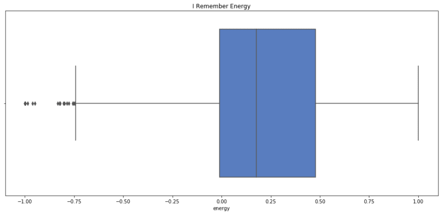
count 133.000000 mean 0.354920 std 0.391389 min -1.000000 25% 0.117536 50% 0.439199 75% 0.639228 max 1.000000 Name: energy, dtype: float64 I remember has a lower mean and median energy, but similar spread to Rock n Roll. I'd say that this fits, as I Remember has almost a melancholic energy, where as Rock n Roll really makes you to get up and move.
What about the zero crossing rate and BPM?
Since zero crossing rate and bpm correlate pretty highly with percussive events, I'd predict that the song with the higher BPM will have a higher zero crossing rate
print 'Rock n Roll average BPM: {}'.format(rnr.bpm.mean()) print 'Rock n Roll average Crossing Rate: {}'.format(rnr.zero_crossing_rate.mean()) print 'I Remember average BPM: {}'.format(i_remember_df.bpm.mean()) print 'I Remember average Crossing Rate: {}'.format(i_remember_df.zero_crossing_rate.mean()) Rock n Roll average BPM: 150.784808472 Rock n Roll average Crossing Rate: 0.14643830815 I Remember average BPM: 136.533708743 I Remember average Crossing Rate: 0.0362864360563 Some scatterplots with spectral centroid on the x axis, and energy on the y axis.
sns.scatterplot(x = rnr.spectral_centroid, y = rnr.energy); plt.show(); sns.scatterplot(x = i_remember_df.spectral_centroid, y = i_remember_df.energy ); plt.show(); 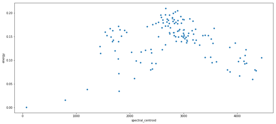
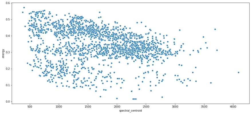
Recall that spectral centroid is where the spectral 'center of mass' is for a given segment. That means that it's picking out the dominant frequency for a segment. I like this because it shows that there's not real relation between the frequency of a segment and its energy. They are both contributing unique information.
build labels and cluster using k means!
song_labels = np.concatenate([np.full((label_len), i) for i, label_len in enumerate([len(rnr), len(i_remember_df)])]) model = sklearn.cluster.KMeans(n_clusters=3) labels = model.fit_predict(features_scaled) plt.scatter(features_scaled.zero_crossing_rate[labels==0], features_scaled.energy[labels==0], c='b') plt.scatter(features_scaled.zero_crossing_rate[labels==1], features_scaled.energy[labels==1], c='r') plt.scatter(features_scaled.zero_crossing_rate[labels==2], features_scaled.energy[labels==2], c='g') plt.xlabel('Zero Crossing Rate (scaled)') plt.ylabel('Energy (scaled)') plt.legend(('Class 0', 'Class 1', 'Class 2')) <matplotlib.legend.Legend at 0x13f054f10> 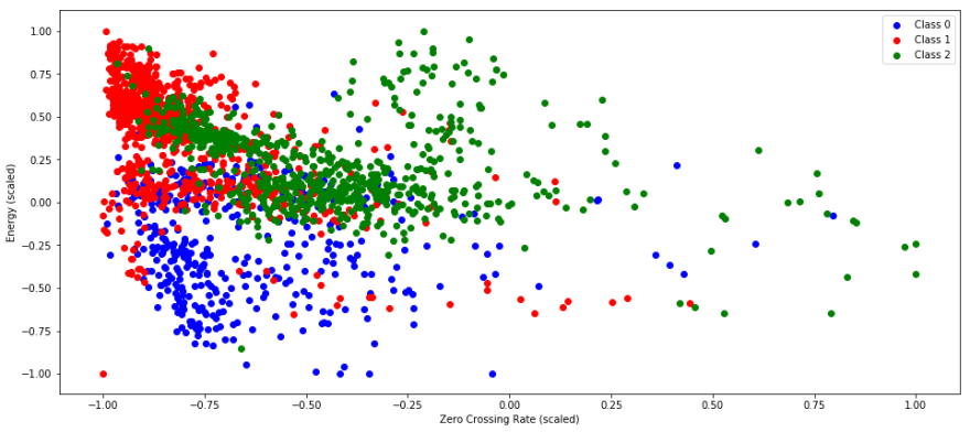
unique_labels, unique_counts = np.unique(model.predict(rnr_scaled), return_counts=True) print unique_counts print 'cluster for rock n roll: ', unique_labels[np.argmax(unique_counts)] [29 9 95] cluster for rock n roll: 2 unique_labels, unique_counts = np.unique(model.predict(i_remember_scaled), return_counts=True) print unique_counts print 'cluster for I remember: ', unique_labels[np.argmax(unique_counts)] [396 877 579] cluster for I remember: 1 I suspect that zero crossing rate and energy are not what the determining factors are for a cluster :)
We can actually listen to the segments that were assigned certain labels
Note that these aren't necessarily consecutive segments
First lets look at I remember
i_remember_clusters = model.predict(i_remember_scaled) label_2_segs = i_remember_segmented['data'][i_remember_clusters==2] label_1_segs = i_remember_segmented['data'][i_remember_clusters==1] label_0_segs = i_remember_segmented['data'][i_remember_clusters==0] Almost all of theses have some of the vocals in them
ipd.Audio(np.concatenate(label_2_segs[:50]), rate = sr) These are the lighter segments, mostly just synths
ipd.Audio(np.concatenate(label_1_segs[:50]), rate = sr) 0 labels seem to be the heavy bass and percussive parts
ipd.Audio(np.concatenate(label_0_segs[:50]), rate = sr) Now Rock n Roll
rnr_clusters = model.predict(rnr_scaled) rock_label_2_segs = rock_n_roll['data'][rnr_clusters==2] rock_label_1_segs = rock_n_roll['data'][rnr_clusters==1] rock_label_0_segs = rock_n_roll['data'][rnr_clusters==0] Again, higher frequencies, vocals included. A lot of consecutive segments included in this class.
ipd.Audio(np.concatenate(rock_label_2_segs[10:40]), rate = sr) <audio controls="controls" > Your browser does not support the audio element. </audio> Lighter sounds, minor key vocals, part of final drum solo
ipd.Audio(np.concatenate(rock_label_1_segs), rate = sr) <audio controls="controls" > Your browser does not support the audio element. </audio> All John Bonham here (only drums). Similar to how in I remember label 0 corresponded to the heavy bass
ipd.Audio(np.concatenate(rock_label_0_segs), rate = sr) <audio controls="controls" > Your browser does not support the audio element. </audio> Conclusion
We've used two very different songs to build vectors of spectral and rhythmic features. We then examined how those features related to each other with boxplots, scatterplots and descriptive statistics. Using those features, we have clustered different segments of the songs together to compare how the different clusters sound together.
More exploration is needed to figure out how to assign a feature value for an entire song that is representative. With more work doing that, it would then be possible to get summary features for entire songs. More on this later!
The rest of this is just some undirected exploring of different features
print rnr_scaled[rnr_clusters==0]['spectral_centroid'].describe() print rnr_scaled[rnr_clusters==1]['spectral_centroid'].describe() print rnr_scaled[rnr_clusters==2]['spectral_centroid'].describe() count 9.000000 mean -0.360693 std 0.250294 min -1.000000 25% -0.370240 50% -0.280334 75% -0.260073 max -0.148394 Name: spectral_centroid, dtype: float64 count 29.000000 mean 0.066453 std 0.363603 min -0.483240 25% -0.211871 50% 0.012854 75% 0.156281 max 0.814435 Name: spectral_centroid, dtype: float64 count 95.000000 mean 0.354971 std 0.261067 min -0.669203 25% 0.218433 50% 0.318239 75% 0.427016 max 1.000000 Name: spectral_centroid, dtype: float64 i_remember_df['mfcc_2'].plot.hist(bins=20, figsize=(14, 5)) <matplotlib.axes._subplots.AxesSubplot at 0x139127290> 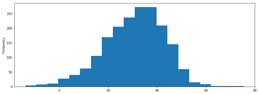
sns.boxplot(x=i_remember_scaled.zero_crossing_rate, palette='muted').set_title('I Remember Zero Crossing Rate'); plt.show(); print i_remember_scaled.zero_crossing_rate.describe() sns.boxplot(rnr_scaled.zero_crossing_rate).set_title('Rock n Roll Zero Crossing Rate'); plt.show(); print rnr_scaled.zero_crossing_rate.describe() 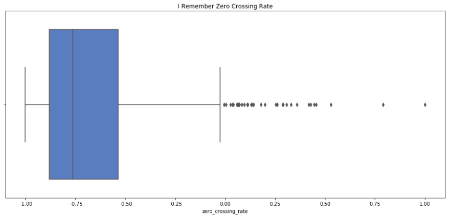
count 1852.000000 mean -0.683760 std 0.255792 min -1.000000 25% -0.880912 50% -0.762325 75% -0.535427 max 1.000000 Name: zero_crossing_rate, dtype: float64 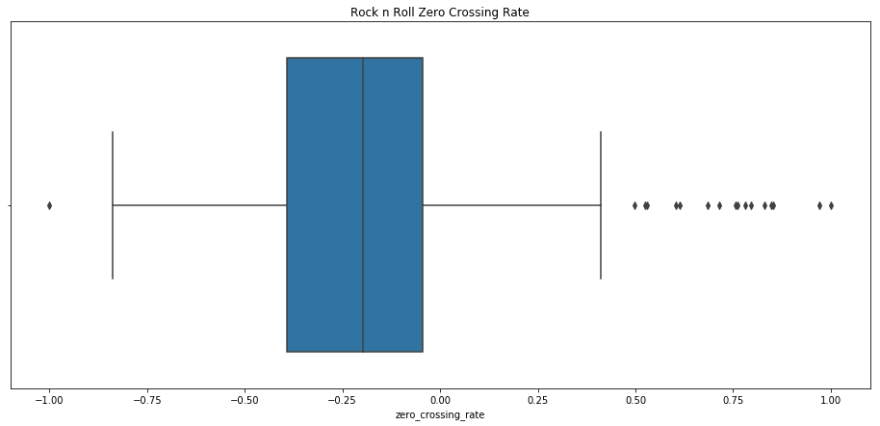
count 133.000000 mean -0.152444 std 0.421004 min -1.000000 25% -0.393116 50% -0.198213 75% -0.045042 max 1.000000 Name: zero_crossing_rate, dtype: float64 print rnr.zero_crossing_rate.describe() print i_remember_df.zero_crossing_rate.describe() count 133.000000 mean 0.146438 std 0.072255 min 0.000977 25% 0.105133 50% 0.138583 75% 0.164871 max 0.344226 Name: zero_crossing_rate, dtype: float64 count 1852.000000 mean 0.036286 std 0.025857 min 0.004319 25% 0.016357 50% 0.028345 75% 0.051281 max 0.206489 Name: zero_crossing_rate, dtype: float64 print rnr.bpm.describe() print i_remember_df.bpm.describe() count 133.000000 mean 150.784808 std 31.793864 min 86.132812 25% 135.999178 50% 135.999178 75% 172.265625 max 287.109375 Name: bpm, dtype: float64 count 1852.000000 mean 136.533709 std 7.140772 min 112.347147 25% 135.999178 50% 135.999178 75% 135.999178 max 258.398438 Name: bpm, dtype: float64 # rnr_scaled['energy'].plot(); i_remember_scaled['energy'].plot(); # rnr_scaled['zero_crossing_rate'].plot(); # rnr_scaled['spectral_centroid'].plot(); # rnr_scaled['mfcc_4'].plot(); plt.show() 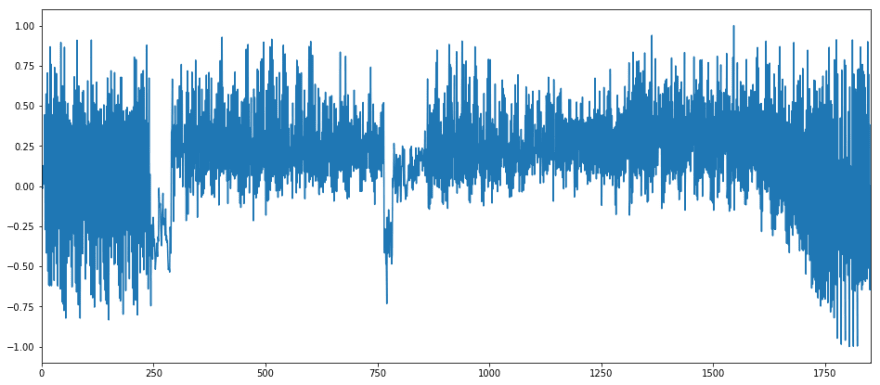
rnr_scaled[['mfcc_' + str(i) for i in xrange(4)]].plot(); plt.show(); 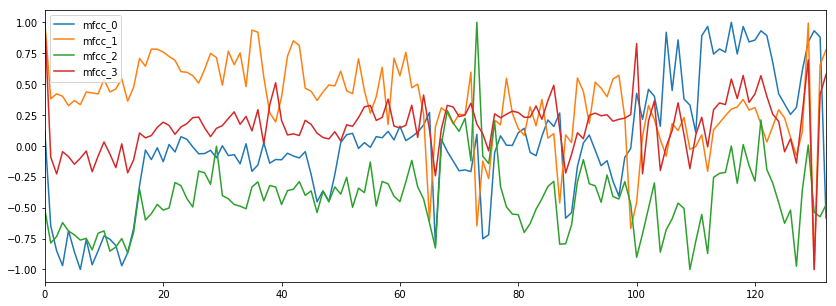
sns.scatterplot(x=rnr_scaled['energy'], y = rnr_scaled['bpm']) <matplotlib.axes._subplots.AxesSubplot at 0x131c69ad0> 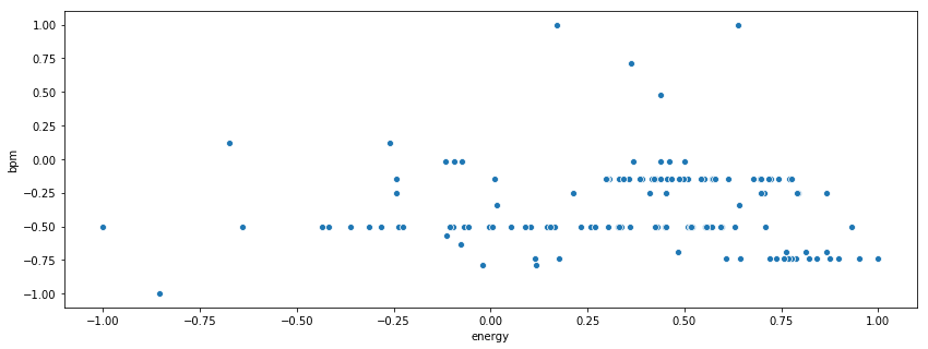
sns.pairplot(rnr_scaled[['mfcc_' + str(i) for i in xrange(5)]], palette='pastel') <seaborn.axisgrid.PairGrid at 0x15f503c10> 

Top comments (0)